一份生物统计数据分析报告

数据背景与分析目的

Cardiotocography (CTG) measures your baby’s heart rate. At the same time it also monitors the contractions in the womb (uterus). CTG is used both before birth (antenatally) and during labour, to monitor the baby for any signs of distress. By looking at various different aspects of the baby’s heart rate, doctors and midwives can see how the baby is coping.

2126 fetal cardiotocograms (CTGs) were automatically processed and the respective diagnostic features measured. The CTGs were also classified by three expert obstetricians and a consensus classification label assigned to each of them. Classification was both with respect to a morphologic pattern (A, B, C. …) and to a fetal state (N, S, P). Therefore the dataset can be used either for 10-class or 3-class experiments.

胎心宫缩图（CTG）测量宝宝的心率。同时，它还监测子宫（子宫）的收缩。CTG在出生前（产前）和分娩期间都用于监测婴儿是否有任何痛苦的迹象。通过观察婴儿心率的各个不同方面，医生和助产士可以看到婴儿是如何应对的。

自动处理 2126 个胎儿胎心宫缩图 （CTG） 并测量相应的诊断特征。CTG还由三名产科专家进行分类，并为每个专家分配一个共识分类标签。分类既有形态学模式（A、B、C….）也有胎儿状态（N、S、P）。因此，该数据集可用于 10 类或 3 类实验。

Cardiotocography数据集包括由专业产科医生分类的心电图上胎儿心率(FHR)和子宫收缩(UC)特征的测量结果。分析该数据集可帮助医生用CTG来诊断婴儿的状态。婴儿的心率。分娩期间婴儿的正常心率在每分钟 110 到 160 次之间。如果婴儿的心率持续偏低或偏高，这可能表明存在问题。婴儿心率的变异性或波动性。如果婴儿的心率在心跳之间略有变化，这是一个好兆头——这表明他们的大脑工作良好。如果他们的心率长时间保持非常相似，这可能表明存在问题。

故本次数据分析报告选取LB,AC,FM,UC,CLASS,NSP这几个变量进行数据分析

数据描述

数据预览

LB	AC	FM	UC	CLASS	NSP
120	0	0	0	9	2
132	4	0	4	6	1
133	2	0	5	6	1
134	2	0	6	6	1
132	4	0	5	2	1
134	1	0	10	8	3
134	1	0	9	8	3

CTG数据

tibble [2,126 × 6] (S3: tbl_df/tbl/data.frame)
 $ LB   : int [1:2126] 120 132 133 134 132 134 134 122 122 122 ...
 $ AC   : int [1:2126] 0 4 2 2 4 1 1 0 0 0 ...
 $ FM   : int [1:2126] 0 0 0 0 0 0 0 0 0 0 ...
 $ UC   : int [1:2126] 0 4 5 6 5 10 9 0 1 3 ...
 $ CLASS: chr [1:2126] "9" "6" "6" "6" ...
 $ NSP  : chr [1:2126] "2" "1" "1" "1" ...

各变量介绍

变量名 |数据	型 |含义	|
LB	连续型变量 |feta	heart rate(FHR)每分钟心跳次数/bpm |
AC	连续型变量 |胎儿加速	跳/bpm |
FM	连续型变量 |每秒胎动	|
UC	连续型变量 |每秒子宫	缩次数 |
CLASS	分类变量 |FHR	模式类代码（1 到 10） |
NSP	分类变量 |胎儿状	类代码（1=正常;2=可疑;3=病理） |

CTG数据

三种胎儿状态下LB、FM和UC的基础统计量

NSP	count	LB_mean	LB_std	AC_mean	AC_std	FM_mean	FM_std	UC_mean	UC_std
1	1655	131.98	9.45	3.42	3.73	6.37	33.83	3.98	2.69
2	295	141.68	7.89	0.21	0.63	7.09	38.24	2.08	2.78
3	176	131.69	9.43	0.33	0.89	15.68	58.20	3.26	3.41

三种胎儿状态下LB、AC、FM和UC的基础统计量

NSP	LB_median	LB_IQR	AC_median	AC_IQR	FM_median	FM_IQR	UC_median	UC_IQR
1	132	13	2	5	0	2	4.0	4
2	143	10	0	0	0	3	1.0	3
3	132	6	0	0	1	2	2.5	5

NSP	LB_min	LB_max	AC_min	AC_max	FM_min	FM_max	UC_min	UC_max
1	106	160	0	26	0	564	0	17
2	120	159	0	6	0	489	0	23
3	110	152	0	4	0	443	0	14

 从表3可观察到健康胎儿的心跳加速度均值明显更大，病理胎儿的宫缩次数均值明显更高

十种FHR模式下LB、FM和UC变量的基础统计量

CLASS	count	LB_mean	LB_std	AC_mean	AC_std	FM_mean	FM_std	UC_mean	UC_std
1	384	132.82	10.76	0.33	0.62	1.12	3.83	3.40	2.79
10	197	142.04	7.84	0.07	0.26	3.31	5.34	1.42	2.08
2	579	132.52	10.07	5.44	3.36	3.98	13.39	3.77	2.44
3	53	129.43	7.60	0.19	0.44	1.94	6.70	1.92	2.34
4	81	133.58	9.21	8.60	3.40	18.06	24.44	3.23	2.63
5	72	141.62	6.51	0.51	0.90	2.38	5.28	3.26	2.90
6	332	130.32	7.76	4.91	3.27	17.03	70.28	5.27	2.91
7	252	132.48	8.34	0.25	0.52	7.36	42.51	4.32	2.42
8	107	128.08	6.85	0.54	1.09	21.62	72.47	5.07	3.17
9	69	137.06	10.39	0.00	0.00	6.48	19.75	0.46	1.05

十种FHR模式下LB、AC、FM和UC的变量的基础统计量

CLASS	LB_median	LB_IQR	AC_median	AC_IQR	FM_median	FM_IQR	UC_median	UC_IQR
1	133.0	17	0	1	0	1	3	4
10	143.0	10	0	0	1	4	0	2
2	132.0	15	5	4	0	2	4	3
3	130.0	11	0	0	0	1	1	3
4	131.0	11	9	4	7	31	3	4
5	142.0	7	0	1	0	1	3	4
6	131.5	11	4	3	0	2	5	4
7	132.0	13	0	0	0	1	4	4
8	130.0	12	0	1	1	1	5	4
9	135.0	19	0	0	1	4	0	0

CLASS	LB_min	LB_max	AC_min	AC_max	FM_min	FM_max	UC_min	UC_max
1	106	159	0	5	0	45	0	23
10	120	159	0	1	0	26	0	9
2	106	160	0	21	0	147	0	11
3	119	146	0	2	0	47	0	10
4	114	158	2	18	0	110	0	11
5	128	159	0	6	0	28	0	11
6	110	146	0	26	0	564	0	16
7	112	156	0	5	0	489	0	12
8	110	140	0	4	0	443	0	14
9	120	152	0	0	0	110	0	6

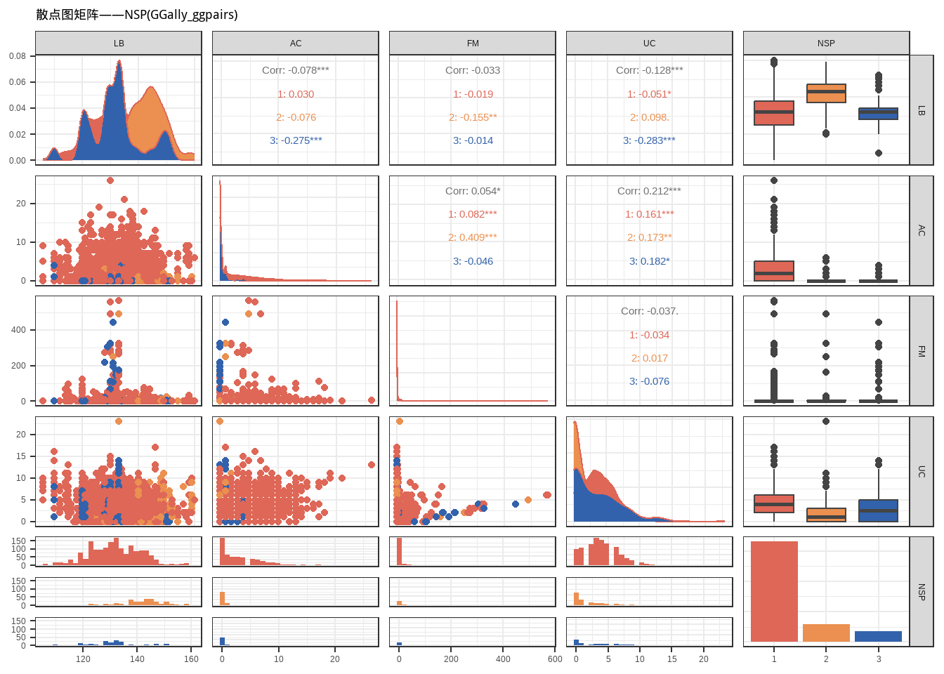
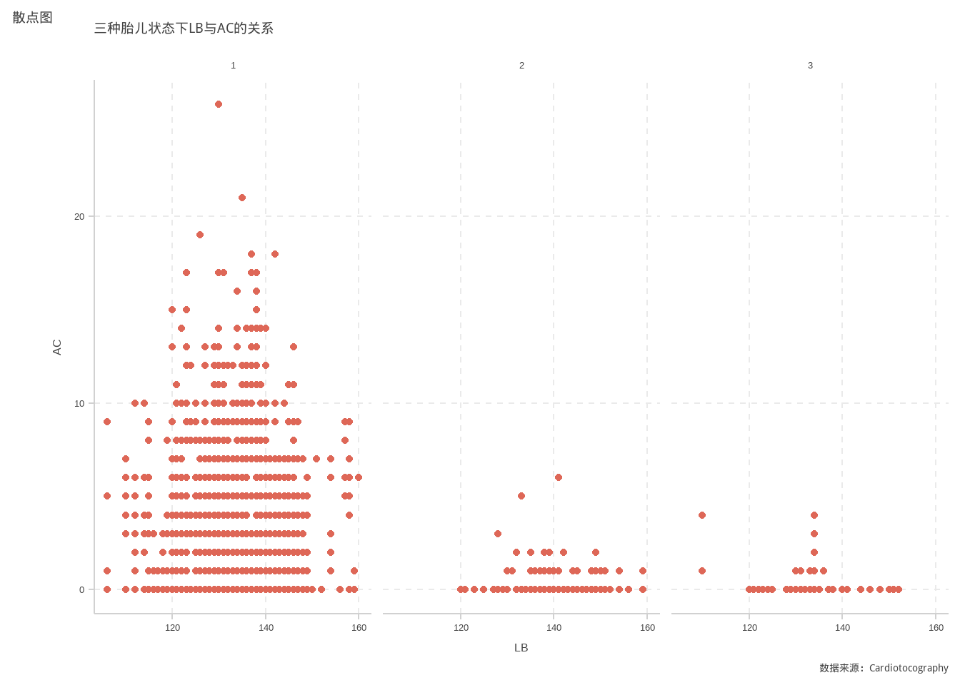
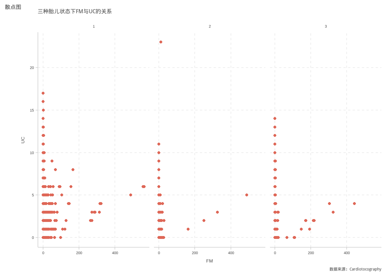
数据可视化

散点图

由图这几种向量并没有明显的相关性

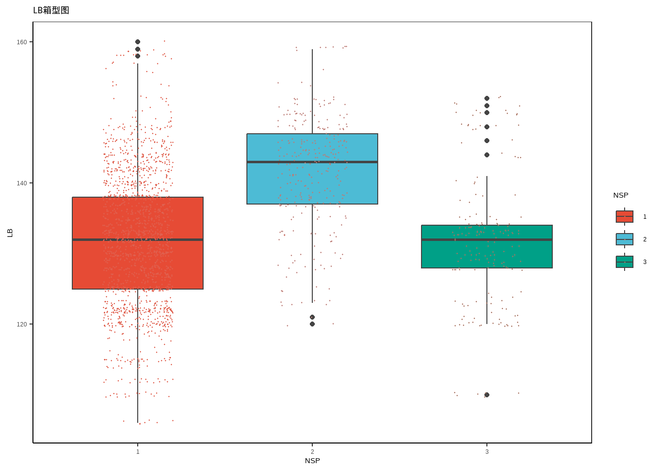
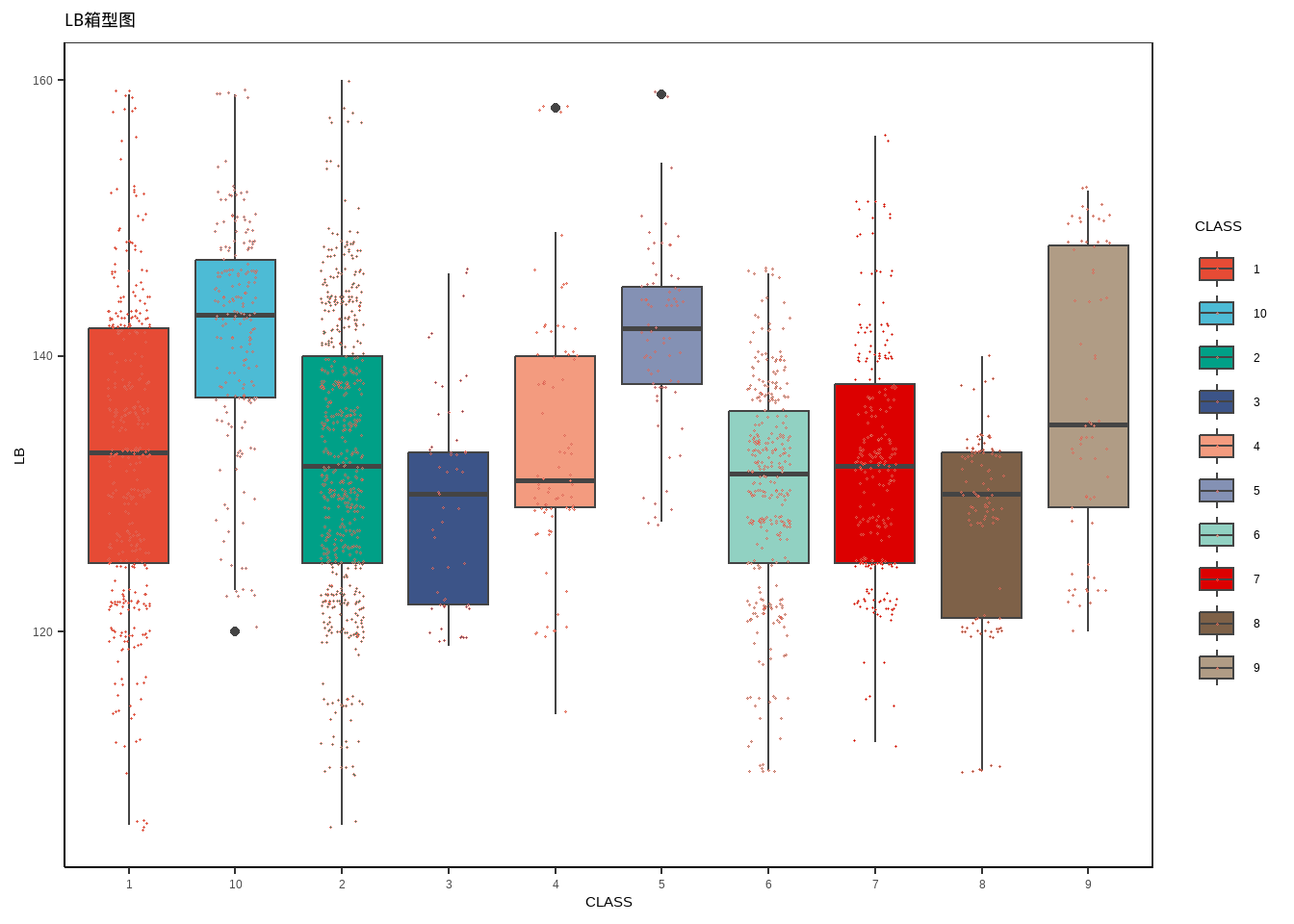
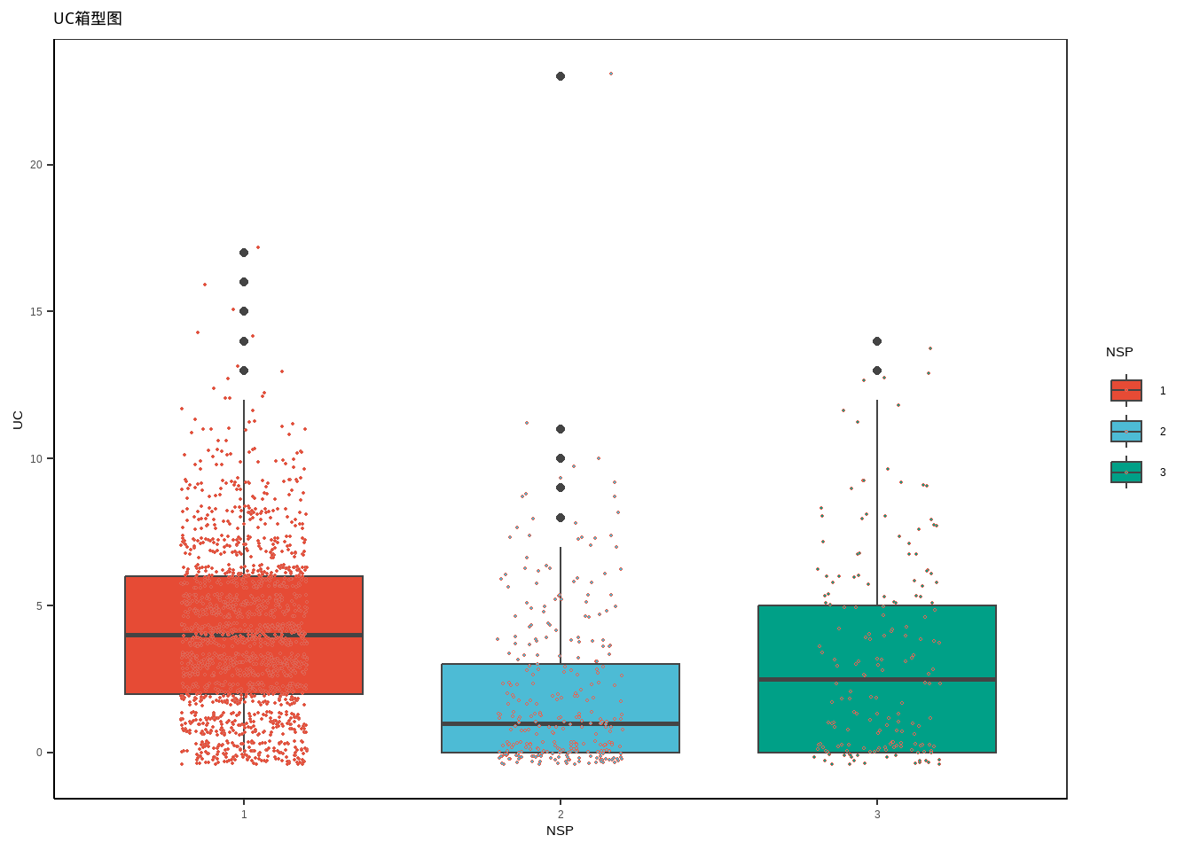
箱形图

注意到三种胎儿状态下正常胎儿心跳偏低，IQR更大

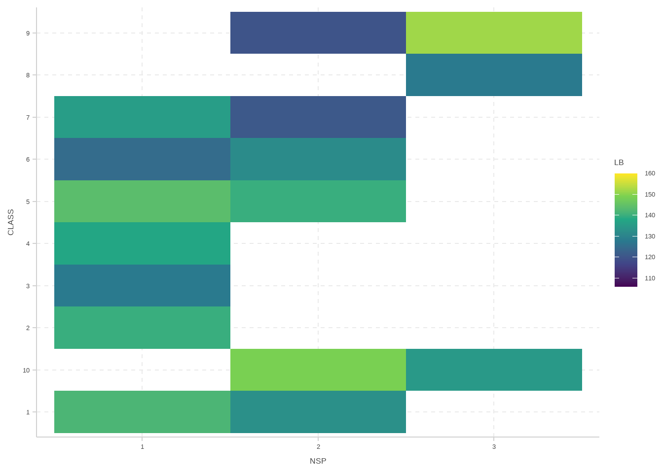
热力图

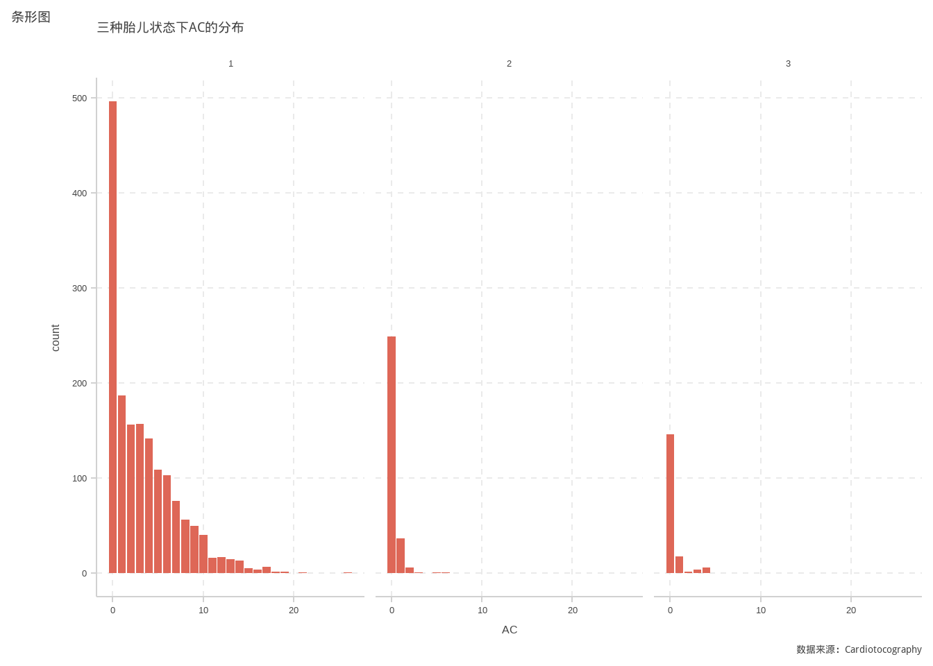
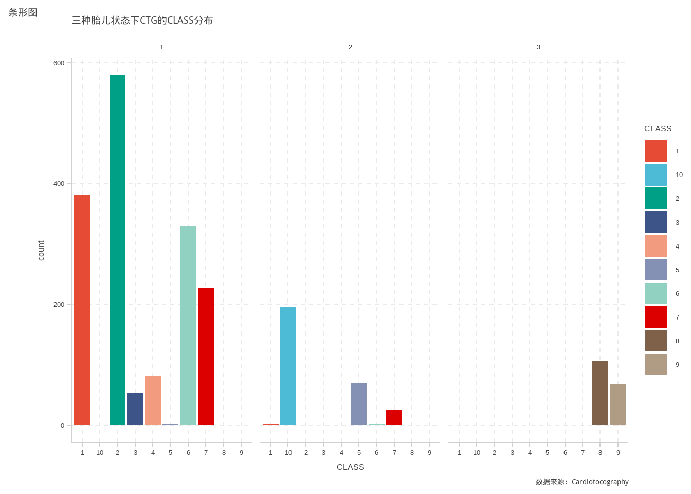
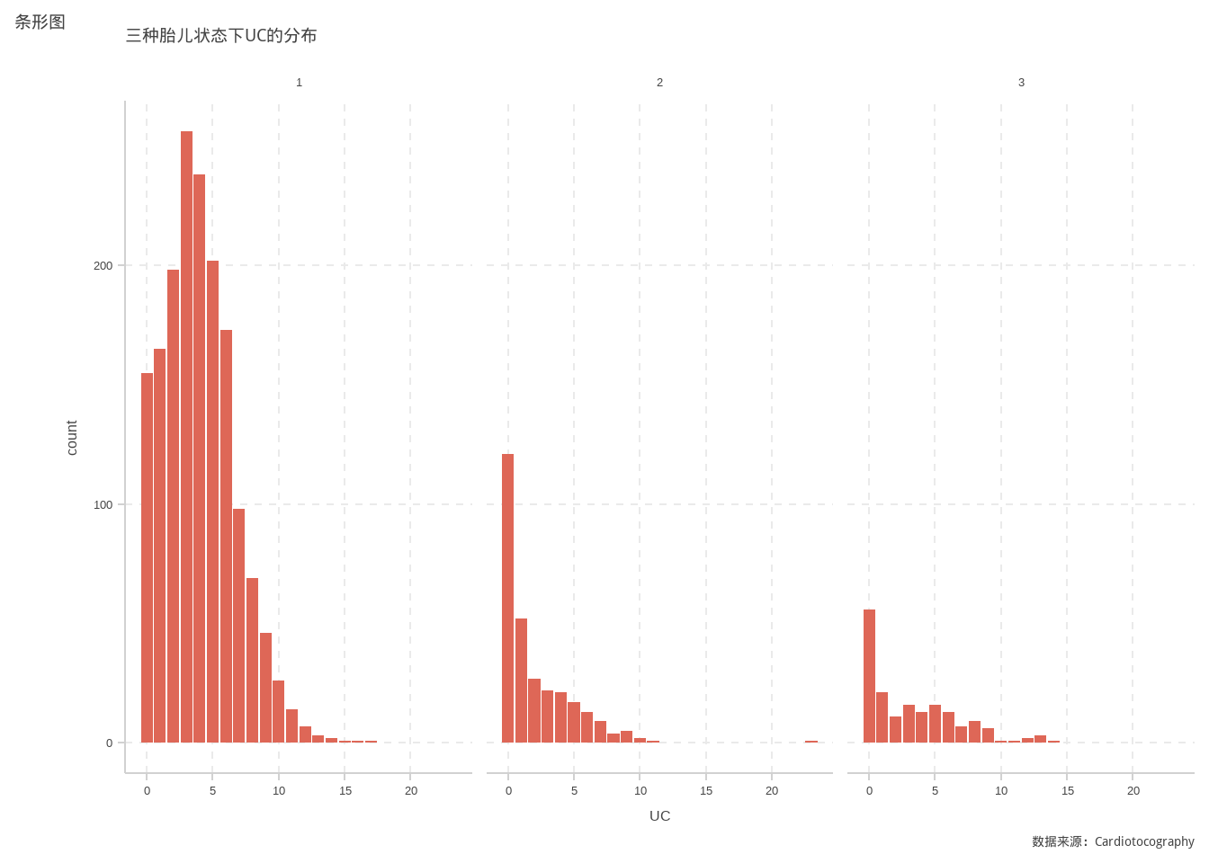
条形图

由图可观察到5，8，9，10类心电图是胎儿危险的信号，推测与UC可能服从泊松分布

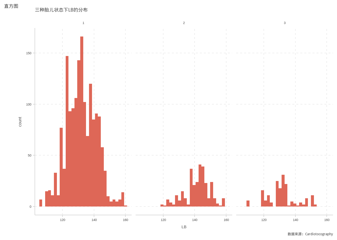
直方图

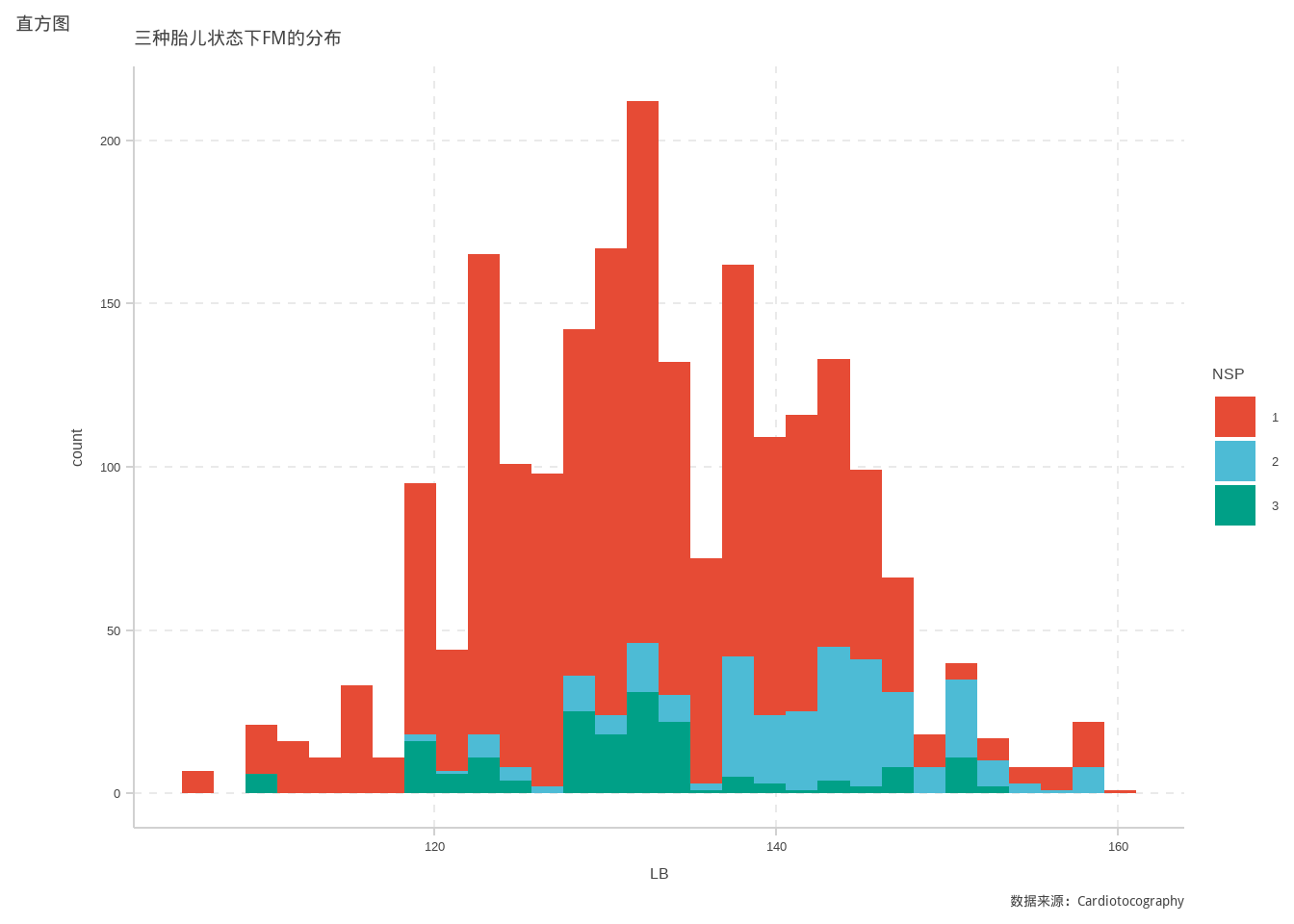
由图可推测LB服从正态分布

假设检验

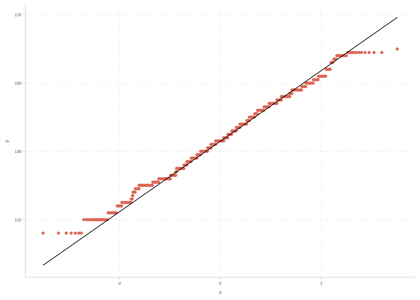
LB变量的正态性检验

QQ图

SW检验

[1] "normal"

    Shapiro-Wilk normality test

data:  .
W = 0.99402, p-value = 3.21e-06

[1] "suspect"

    Shapiro-Wilk normality test

data:  .
W = 0.97297, p-value = 2.341e-05

[1] "pathologic"

    Shapiro-Wilk normality test

data:  .
W = 0.94487, p-value = 2.517e-06

t检验

[1] "normal"

    One Sample t-test

data:  .
t = 567.9, df = 1654, p-value < 2.2e-16
alternative hypothesis: true mean is not equal to 0
95 percent confidence interval:
 131.5260 132.4377
sample estimates:
mean of x 
 131.9819 

[1] "suspect"

    One Sample t-test

data:  .
t = 308.47, df = 294, p-value < 2.2e-16
alternative hypothesis: true mean is not equal to 0
95 percent confidence interval:
 140.7808 142.5887
sample estimates:
mean of x 
 141.6847 

[1] "pathologic"

    One Sample t-test

data:  .
t = 185.2, df = 175, p-value < 2.2e-16
alternative hypothesis: true mean is not equal to 0
95 percent confidence interval:
 130.2842 133.0908
sample estimates:
mean of x 
 131.6875 

lillie检验

    Lilliefors (Kolmogorov-Smirnov) normality test

data:  .
D = 0.043589, p-value = 9.23e-08


    Lilliefors (Kolmogorov-Smirnov) normality test

data:  .
D = 0.091628, p-value = 2.907e-06


    Lilliefors (Kolmogorov-Smirnov) normality test

data:  .
D = 0.15885, p-value = 1.036e-11

由以上几种正态性检验均可在显著性水平>0.001下说明LB即胎儿每分钟心跳数服从正态分布

正常与病理胎儿状态LB均值齐性t检验

    Welch Two Sample t-test

data:  d1$LB and d3$LB
t = 0.39352, df = 214.13, p-value = 0.6943
alternative hypothesis: true difference in means is not equal to 0
95 percent confidence interval:
 -1.180125  1.768871
sample estimates:
mean of x mean of y 
 131.9819  131.6875 

可见两者均值应该相等

正常与病理胎儿状态LB方差齐性F检验

    F test to compare two variances

data:  d1$LB and d2$LB
F = 1.4362, num df = 1654, denom df = 294, p-value = 0.0001161
alternative hypothesis: true ratio of variances is not equal to 1
95 percent confidence interval:
 1.198262 1.702818
sample estimates:
ratio of variances 
          1.436249 

可见在显著性水平>0.001下应该拒绝原假设，认为两者方差不等

各变量间的相关性检验

pearson

[1] -3.593255
[1] 2124
[1] 0.0001670021

spearman

    Pearson's product-moment correlation

data:  d$LB and d$AC
t = -3.6042, df = 2124, p-value = 0.0003203
alternative hypothesis: true correlation is not equal to 0
95 percent confidence interval:
 -0.12008107 -0.03557304
sample estimates:
        cor 
-0.07796711 

两者负相关

##AC变量泊松分布pearson和似然比检验

   Var1 Freq
1     0  891
2     1  242
3     2  164
4     3  162
5     4  148
6     5  110
7     6  104
8     7   76
9     8   56
10    9   50
11   10   40
12   11   16
13   12   17
14   13   15
15   14   13
16   15    5
17   16    4
18   17    7
19   18    2
20   19    2
21   21    1
22   26    1
[1] 8371.625
[1] 0

离群值检验

    chi-squared test for outlier

data:  d$LB
X-squared = 7.6981, p-value = 0.005528
alternative hypothesis: lowest value 106 is an outlier

结论与建议

当妇科医生观看胎儿的CTG即心肺宫缩图时，胎儿心跳加速是胎儿健康的放心讯号,类型为5,8,9,10的心电图是危险信号，应该慎重诊断

附录

library(tidyverse)
library(knitr)
library(kableExtra)
library(ggsci)
library(nortest)
library(GGally)
library(outliers)

d=read.csv("data/CTG.csv",header=T)
d <- as.tibble(d) 
d <- select(d,LB,AC,FM,UC,CLASS,NSP)
d$CLASS <- as.character(d$CLASS );d$NSP <- as.character(d$NSP )
df <- tibble("变量名"=c("LB","AC","FM","UC","CLASS","NSP"),
             "数据类型"=c(rep("连续型变量",times=4),"分类变量","分类变量"),
             "含义"=c("fetal heart rate(FHR)每分钟心跳次数/bpm",
                    "胎儿加速心跳/bpm",
                    "每秒胎动数",
                    "每秒子宫收缩次数",
                    "FHR 模式类代码（1 到 10）",
                    "胎儿状态类代码（1=正常;2=可疑;3=病理）"
             ))

d %>% head(7) %>% 
  kable( booktabs = TRUE,caption = "CTG数据") %>% 
  kable_styling(bootstrap_options = "bordered") %>% 
  row_spec(0, color = "white", background = "#696969" )
str(d)

df %>% 
  kable( booktabs = TRUE,caption = "CTG数据") %>% 
  kable_styling(bootstrap_options = "bordered") %>% 
  row_spec(0, color = "black", background = "#98F5FF" )

bind_cols(
  d |>
    group_by(NSP) |>
    summarise(count = n()),
  d %>% group_by(NSP) |>
    summarise(across(
      c("LB","AC","FM","UC"),
      list( 
        mean = \(x) mean(x, na.rm=TRUE), 
        std = \(x) sd(x, na.rm=TRUE)
        
      )) ) %>% select(-NSP)) %>% 
  knitr::kable(digits=2,caption="三种胎儿状态下LB、AC、FM和UC的基础统计量")%>% 
  kable_styling(bootstrap_options = "bordered") %>% 
  row_spec(0, color = "black", background = "#98F5FF" )

d %>% group_by(NSP) |>
  summarise(across(
    c("LB","AC","FM","UC"),
    list( 
      median = \(x) median(x, na.rm=TRUE),
      IQR =\(x) IQR(x, na.rm=TRUE)
    )))   %>% 
  knitr::kable(digits=2)%>% 
  kable_styling(bootstrap_options = "bordered") %>% 
  row_spec(0, color = "black", background = "#98F5FF" )

d %>% group_by(NSP) |>
  summarise(across(
    c("LB","AC","FM","UC"),
    list( 
      min = \(x) min(x, na.rm=TRUE), 
      max = \(x) max(x, na.rm=TRUE)
      
    )))   %>% 
  knitr::kable(digits=2)%>% 
  kable_styling(bootstrap_options = "bordered") %>% 
  row_spec(0, color = "black", background = "#98F5FF" )

bind_cols(
  d |>
    group_by(CLASS) |>
    summarise(count = n()),
  d %>% group_by(CLASS) |>
    summarise(across(
      c("LB","AC","FM","UC"),
      list( 
        mean = \(x) mean(x, na.rm=TRUE), 
        std = \(x) sd(x, na.rm=TRUE)
        
      )) ) %>% select(-CLASS)) %>% 
  knitr::kable(digits=2,caption="十种FHR模式下LB、AC、FM和UC的变量的基础统计量")%>% 
  kable_styling(bootstrap_options = "bordered") %>% 
  row_spec(0, color = "black", background = "#98F5FF" )

d %>% group_by(CLASS) |>
  summarise(across(
    c("LB","AC","FM","UC"),
    list( 
      median = \(x) median(x, na.rm=TRUE),
      IQR =\(x) IQR(x, na.rm=TRUE)
    )))   %>% 
  knitr::kable(digits=2)%>% 
  kable_styling(bootstrap_options = "bordered") %>% 
  row_spec(0, color = "black", background = "#98F5FF" )

d %>% group_by(CLASS) |>
  summarise(across(
    c("LB","AC","FM","UC"),
    list( 
      min = \(x) min(x, na.rm=TRUE), 
      max = \(x) max(x, na.rm=TRUE)
      
    )))   %>% 
  knitr::kable(digits=2)%>% 
  kable_styling(bootstrap_options = "bordered") %>% 
  row_spec(0, color = "black", background = "#98F5FF" )

d %>% select(-CLASS) %>% ggpairs( columns=1:5, aes(color=NSP)) + 
  ggtitle("散点图矩阵——NSP(GGally_ggpairs)")+
  theme_bw() 

ggplot(d,aes(NSP,LB))+
  geom_boxplot(mapping=aes(fill=NSP))+
  geom_jitter(aes(fill=NSP),width =0.2,shape = 21,size=0.2)+
  theme_bw() + 
  theme(panel.grid.major =element_blank(), 
        panel.grid.minor = element_blank(),
        panel.background = element_blank(),
        axis.line = element_line(colour = "black"))+
  scale_fill_npg()+
  ggtitle("LB箱型图")

ggplot(d,aes(CLASS,LB))+
  geom_boxplot(mapping=aes(fill=CLASS))+
  geom_jitter(aes(fill=CLASS),width =0.2,shape = 21,size=0.2)+
  theme_bw() + 
  theme(panel.grid.major =element_blank(), 
        panel.grid.minor = element_blank(),
        panel.background = element_blank(),
        axis.line = element_line(colour = "black"))+
  scale_fill_npg()+
  ggtitle("LB箱型图")

ggplot(d,aes(NSP,UC))+
  geom_boxplot(mapping=aes(fill=NSP))+
  geom_jitter(aes(fill=NSP),width =0.2,shape = 21,size=0.3)+
  theme_bw() + 
  theme(panel.grid.major =element_blank(), 
        panel.grid.minor = element_blank(),
        panel.background = element_blank(),
        axis.line = element_line(colour = "black"))+
  scale_fill_npg()+
  ggtitle("UC箱型图")


ggplot(d, aes(
  x = NSP, y = CLASS,fill=LB)) +
  geom_tile() +
  scale_fill_viridis_c()

ggplot(d)+
  geom_bar(mapping=aes(x=AC,fill=AC))+
  facet_wrap(~NSP)+
  labs(title = "三种胎儿状态下AC的分布",
       tag = "条形图",
       caption = "数据来源：Cardiotocography")+
  scale_fill_npg()


ggplot(d)+
  geom_bar(mapping=aes(x=CLASS,fill=CLASS))+
  facet_wrap(~NSP)+
  labs(title = "三种胎儿状态下CTG的CLASS分布",
       tag = "条形图",
       caption = "数据来源：Cardiotocography")+
  scale_fill_npg()



ggplot(d)+
  geom_bar(mapping=aes(x=UC,fill=UC))+
  facet_wrap(~NSP)+
  labs(title = "三种胎儿状态下UC的分布",
       tag = "条形图",
       caption = "数据来源：Cardiotocography")+
  scale_fill_npg()

ggplot(d)+
  geom_histogram(mapping=aes(x=LB))+
  facet_wrap(~NSP)+
  labs(title = "三种胎儿状态下LB的分布",
       tag = "直方图",
       caption = "数据来源：Cardiotocography")

ggplot(d)+
  geom_histogram(mapping=aes(x=FM))+
  facet_wrap(~NSP)+
  labs(title = "三种胎儿状态下LB的分布",
       tag = "直方图",
       caption = "数据来源：Cardiotocography")

ggplot(d)+
  geom_histogram(mapping=aes(x=LB,fill=NSP))+
  labs(title = "三种胎儿状态下FM的分布",
       tag = "直方图",
       caption = "数据来源：Cardiotocography")+
  scale_fill_npg()

ggplot(d)+
  geom_histogram(mapping=aes(x=LB))+
  facet_wrap(~CLASS)+
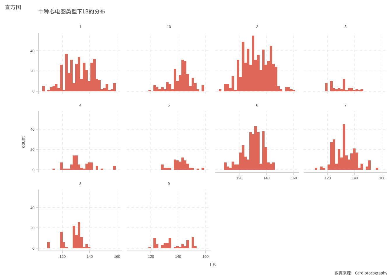
  labs(title = "十种心电图类型下LB的分布",
       tag = "直方图",
       caption = "数据来源：Cardiotocography")+
  scale_fill_npg()

d %>% ggplot(aes(sample =LB )) +
  geom_qq() + geom_qq_line()

"normal";
(d %>% filter(NSP=="1"))$LB %>% shapiro.test()

"suspect";
(d %>% filter(NSP=="2"))$LB %>% shapiro.test()

"pathologic";
(d %>% filter(NSP=="3"))$LB %>% shapiro.test()

"normal";
(d %>% filter(NSP=="1"))$LB %>% t.test()

"suspect";
(d %>% filter(NSP=="2"))$LB %>% t.test()

"pathologic";
(d %>% filter(NSP=="3"))$LB %>% t.test()

d1=d %>% filter(NSP=="1")
d2=d %>% filter(NSP=="2")
d3=d %>% filter(NSP=="3")
d1$LB %>% lillie.test()
d2$LB %>% lillie.test()
d3$LB %>% lillie.test()

t.test(d1$LB,d3$LB)

var.test(d1$LB,d2$LB)

x=d$LB;y=d$AC;
n=length(x)
r=sum((x-mean(x))*(y-mean(y)))/sqrt(sum((x-mean(x))^2)*sum((y-mean(y))^2))
pearson=r*sqrt(n-2/1-r^2)
pearson
n-2
pt(pearson,n-2)


cor.test(d$LB,d$AC)


as.data.frame(table(d$AC))

Ob=(head(as.data.frame(table(d$AC)),10))$Freq;n=sum(Ob);lambda=t(0:9)%*%Ob/n
p=exp(-lambda)*lambda^(0:9)/factorial(0:9)
E=p*n;Q=sum((E-Ob)^2/E);pvalue=pchisq(Q,8,low=F)
Q
pvalue

chisq.out.test(d$LB)