---
title: non-parametric
author: 'Kili'
date: "2023-12-05"
categories: ["R",'非参数']
toc: true
cache: true
---
> *吾生也有涯,而知也无涯,以有涯随无涯,殆已。*
# 数据描述与背景导入
```{r include=FALSE}
d <- read.csv("C:/Users/10156/Desktop/non/data/winequality-red.csv", sep=";")
library(tidyverse)
library(knitr)
library(kableExtra)
library(ggsci)
library(nortest)
library(GGally)
library(outliers)
library(corrplot)
library(DescTools)
library(ks)
library(caret)
df <- tibble("变量名"=c("fixed acidity", "volatile acidity",
"citric acid", "residual sugar", "chlorides",
"free sulfur dioxide", "total sulfur dioxide", "density", "pH", "sulphates",
"alcohol", "quality"),
"数据类型"=c(rep("连续型变量",times=11),"有序分类变量"),
"含义"=c("固定酸度","挥发性酸度",
"柠檬酸", "残糖", "氯化物", "游离二氧化硫",
"总二氧化硫", "密度", "pH值", "硫酸盐",
"酒精浓度", "酒质量3-8")
)
knitr::opts_chunk$set(echo = FALSE, warning = FALSE)
```
## 各变量介绍
```{r}
df %>%
kable( booktabs = TRUE,caption = "CTG数据") %>%
  kable_styling(bootstrap_options = "bordered") %>%
  row_spec(0, color = "black", background = "#98F5FF" )
```
## 数据预览
```{r}
d %>%
  mlmCorrs::corstars()
```
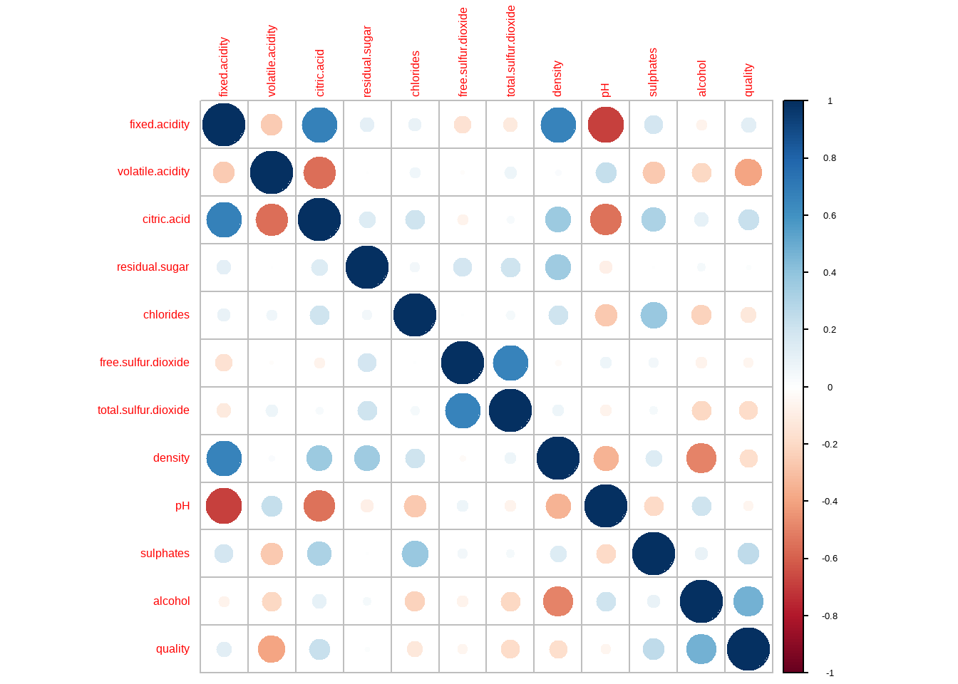
```{r}
corrplot(corr=cor(d))
d$quality=factor(d$quality,ordered=TRUE)
d %>% select(1:6)%>% head(5) %>%
kable( booktabs = TRUE,caption = "CTG数据") %>%
  kable_styling(bootstrap_options = "bordered") %>%
  row_spec(0, color = "white", background = "#696969" )
d %>% select(7:12)%>% head(5) %>%
kable( booktabs = TRUE,caption = "CTG数据") %>%
  kable_styling(bootstrap_options = "bordered") %>%
  row_spec(0, color = "white", background = "#696969" )
skimr::skim(d)
```
# 可视化
```{r}
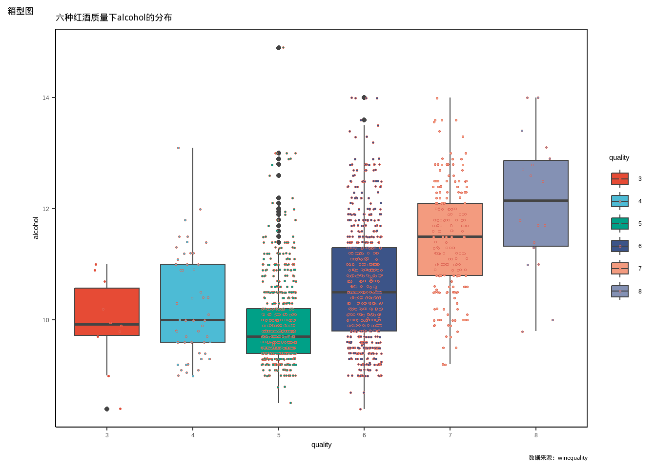
ggplot(d,aes(quality,alcohol))+
geom_boxplot(mapping=aes(fill=quality))+
geom_jitter(aes(fill=quality),width =0.2,shape = 21,size=0.5)+
theme_bw() +
theme(panel.grid.major =element_blank(),
panel.grid.minor = element_blank(),
panel.background = element_blank(),
axis.line = element_line(colour = "black"))+
scale_fill_npg()+
labs(title = "六种红酒质量下alcohol的分布",
tag = "箱型图",
caption = "数据来源:winequality")
```
\newpage
# 非参数检验
## 多样本位置检验:六种质量下的红酒酒精浓度中位数是否不同?
$$
H_0:same\ vs\ H_1:not
$$
```{r}
kruskal.test(alcohol~quality,d)
```
$$
H_0:same\ vs\ H_1:increasing
$$
```{r}
JonckheereTerpstraTest( alcohol~quality,data=d,alternative = c( "increasing"))
```
\newpage
## 独立两样本比较的Wilcoxon秩和检验
将红酒分成两组, 比较质量为3,4,5与6,7,8的红酒样本的酒精浓度中位数是否有显著性 差异
$$
\\H_0:\Delta=0
$$
```{r}
d1 <- d %>% filter(quality==5|quality==4|quality==3)
d2 <- d %>% filter(quality==6|quality==7|quality==8)
wilcox.test(d1$alcohol,d2$alcohol)
```
检验结果可见两组中位数确实有显著性差异
## 相关性检验
$$
H_0:unrelated\ vs\ H_1:related
$$
### spearman
```{r}
cor.test(d$alcohol,as.numeric(d$quality),meth="spearman")
```
### Kendall
将酒精浓度转化为有序类别变量
$$
Kendall's \ \tau_b\\\
$$
```{r}
cor.test(d$alcohol,as.numeric(d$quality),meth="kendall")
```
## 分布检验
```{r}
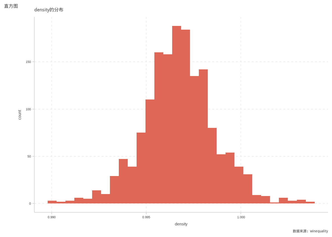
ggplot(d)+
geom_histogram(mapping=aes(x=density))+
labs(title = "density的分布",
tag = "直方图",
caption = "数据来源:winequality")
```
## 红酒密度的分布是否符合正态
$$
H_0:norm\ vs\ H_1:unnorm
$$
```{r}
x <- d$density
mu=mean(x);sigma=sum((x-mean(x))^2)/length(x)
ks.test(x,"pnorm",mu,sigma)
```
接下来比较一下先前分出的两组红酒的酒精浓度分布是否不同
$$
H_0:same\ pdf\ vs\ H_1:unsame
$$
```{r}
ks.test(d1$alcohol,d2$alcohol)
```
\newpage
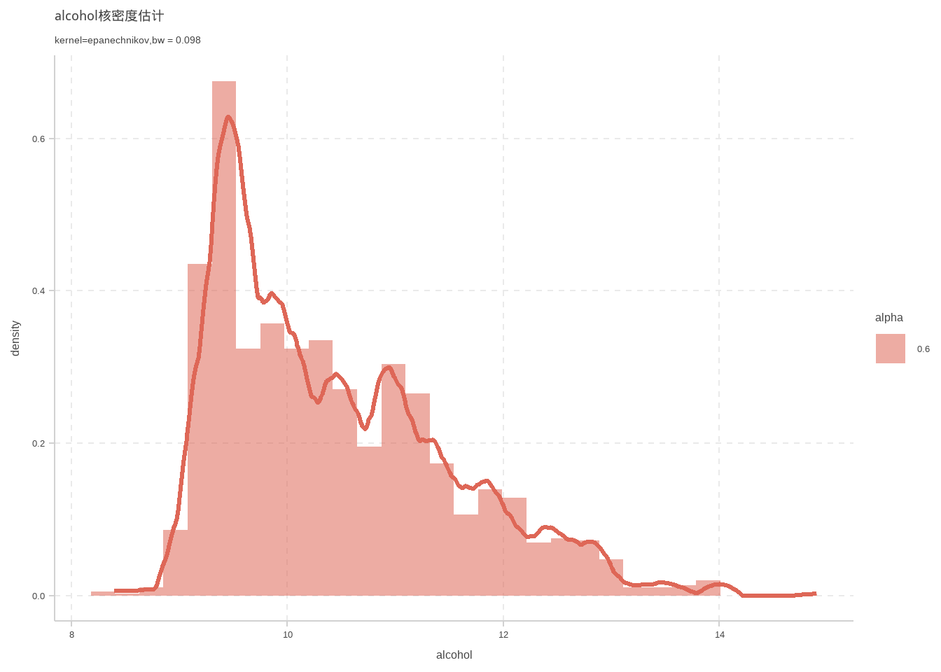
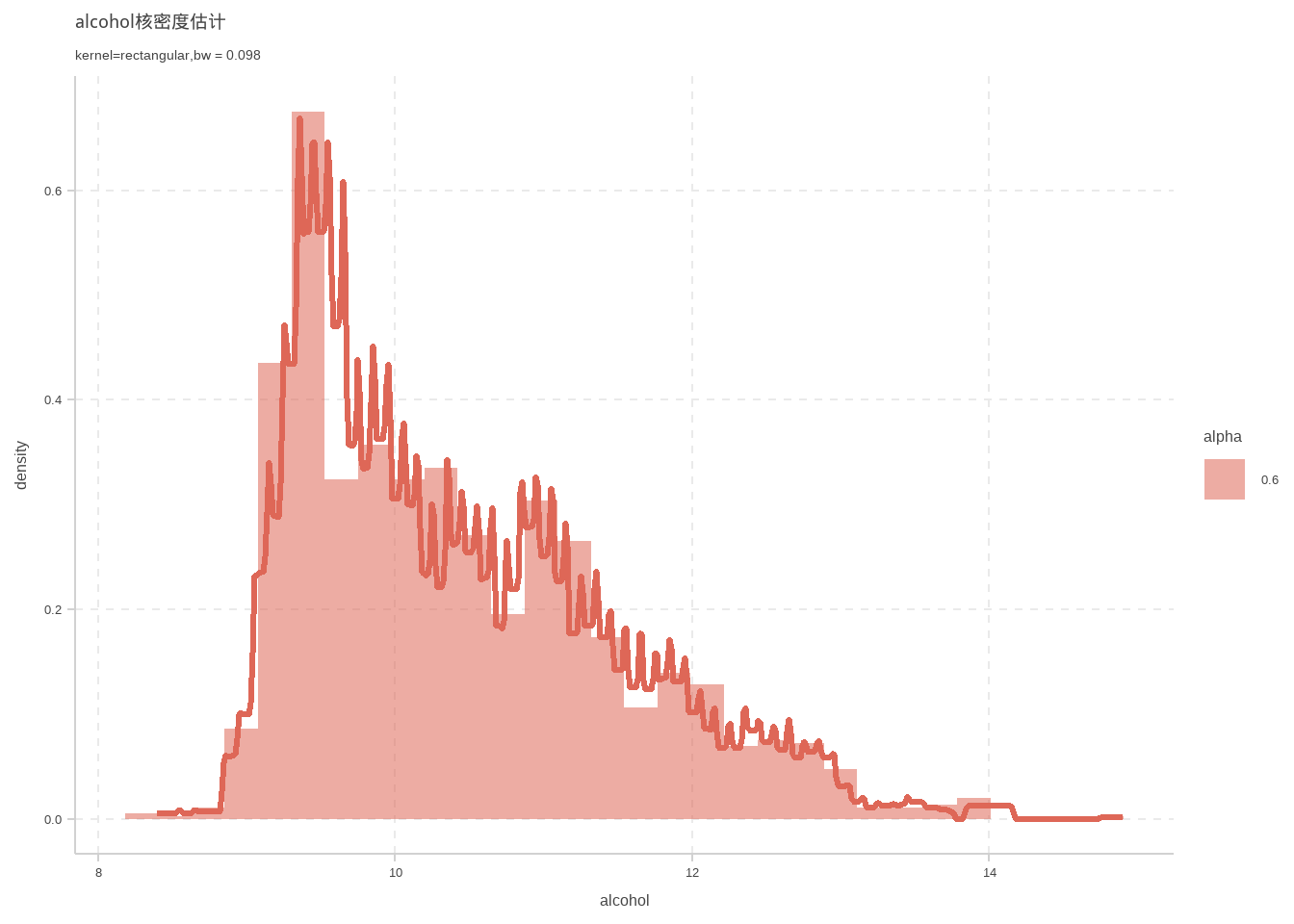
# 一元核密度估计
这里使用插入法计算宽窗
```{r}
d %>% ggplot(aes(x = alcohol)) +geom_density(kernel ="gaussian",size=1.1,bw=bw.SJ(d$alcohol))+labs(
  title = "alcohol核密度估计",
  subtitle = "kernel=gaussian,bw = 0.098"
)+geom_histogram(mapping = aes(y = ..density..,alpha = 0.6))

d %>% ggplot(aes(x = alcohol)) +geom_density(kernel ="epanechnikov",size=1.1,bw=bw.SJ(d$alcohol))+labs(
  title = "alcohol核密度估计",
  subtitle = "kernel=epanechnikov,bw = 0.098"
)+geom_histogram(mapping = aes(y = ..density..,alpha = 0.6))

d %>% ggplot(aes(x = alcohol)) +geom_density(kernel ="rectangular",size=1.1,bw=bw.SJ(d$alcohol))+labs(
  title = "alcohol核密度估计",
  subtitle = "kernel=rectangular,bw = 0.098"
)+geom_histogram(mapping = aes(y = ..density..,alpha = 0.6))
```
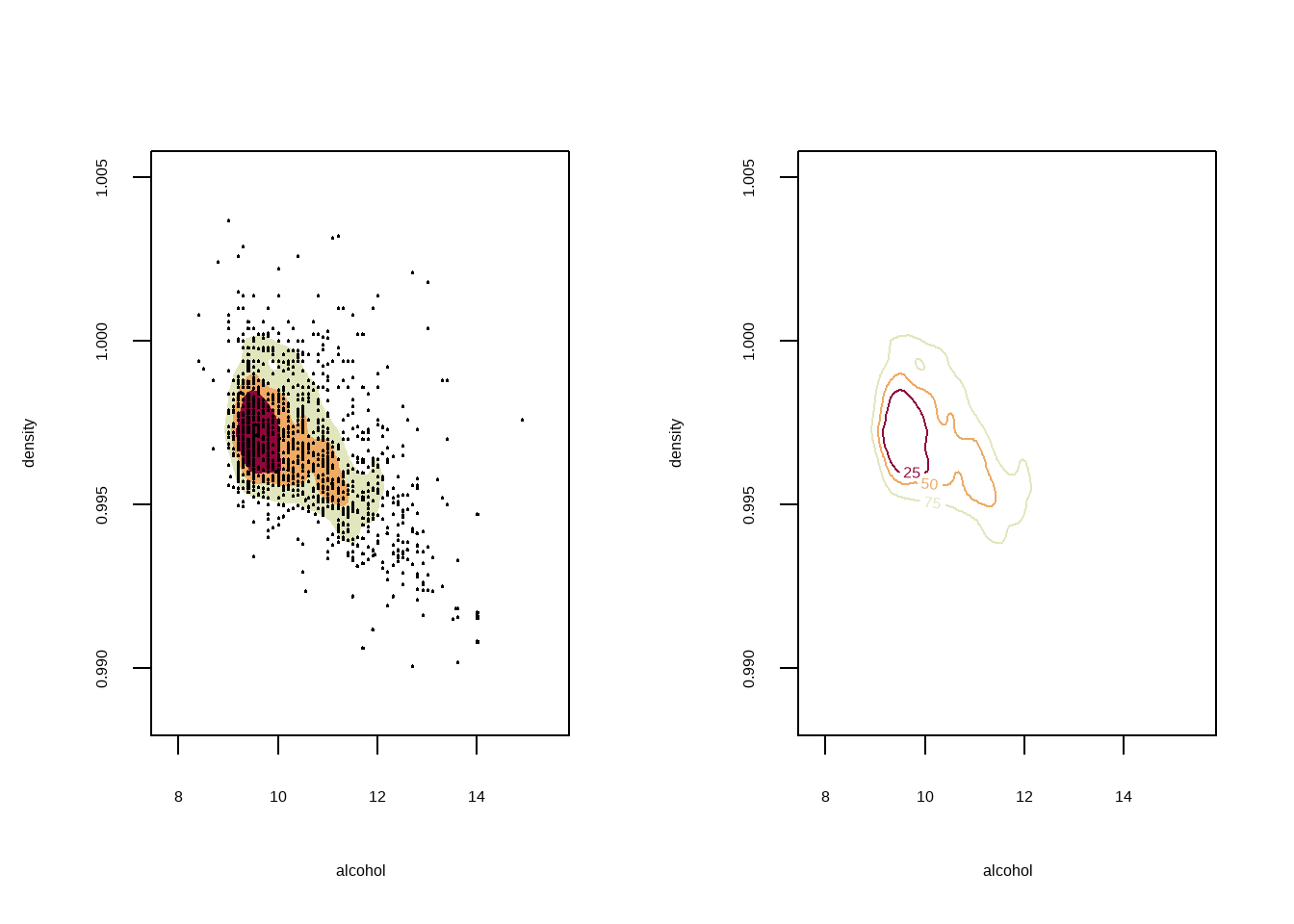
## 多元核密度估计
对酒精浓度与密度做二元核密度估计
```{r}
par(mfrow=c(1,2))
fhat <- kde(d %>% select(alcohol,density))
plot(fhat,display="filled.contour2")
points(d %>% select(alcohol,density),cex=0.1,pch=5)
plot(fhat,diplay="persp")
```
\newpage
# 分类
先分好训练集与测试集,且要保证好酒与坏酒的比例与原数据集相近
```{r}
d <- read.csv("C:/Users/10156/Desktop/non/data/winequality-red.csv", sep=";")
d$quality[d$quality==3]=0
d$quality[d$quality==4]=0
d$quality[d$quality==5]=0
d$quality[d$quality==6]=1
d$quality[d$quality==7]=1
d$quality[d$quality==8]=1
d$quality=factor(d$quality)
library(rsample)
d_split <- initial_split(d, prop = 0.9,strata = quality)
d_train <- training(d_split)
d_test <- testing(d_split)
```
## logistic回归
$$
cheap\ wine1(3,4,5)and\ good\ wine2(6,7,8)res\\
\begin{aligned}
Y \sim & B(m, p) \\
g(p) =& \beta_0 + \beta_1 x_1 + \dots + \beta_k x_k \\
AIC\ backward\ to\ choose\ model
\end{aligned}
$$
```{r }
fit=glm(quality~fixed.acidity + volatile.acidity + citric.acid + residual.sugar +
chlorides + free.sulfur.dioxide + total.sulfur.dioxide +
density + pH + sulphates + alcohol,family = binomial,data=d_train,na.action = na.pass)
fit1=step(fit,direction = "backward")
```
```{r}
summary(fit1)
```
模型预测:
```{r}
plot_confusion = function(cm) {
  as.table(cm) %>%
    as_tibble() %>%
    mutate(response = factor(response),
           truth = factor(truth, rev(levels(response)))) %>%
    ggplot(aes(response, truth, fill = n)) +
    geom_tile() +
    geom_text(aes(label = n)) +
    scale_fill_gradientn(colors = rev(hcl.colors(10, "Blues")), breaks = seq(0,10,2)) +
    coord_fixed() +
    theme_minimal()
}

# 测试数据真实值
truth <- d_test$quality
# 测试数据预测值
pred <- predict.glm(fit1,newdata = d_test,type="response")
pred[pred>0.5]=1
pred[pred<0.5]=0
# 计算混淆矩阵
confusionMatrix(table(pred,truth))
```
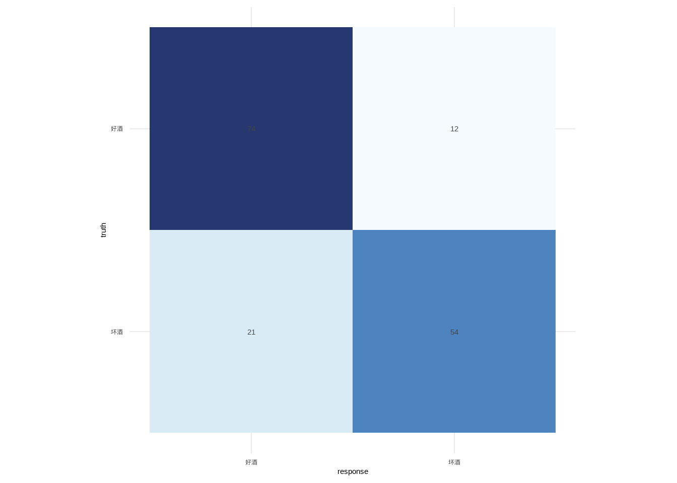
## KNN
```{r}
library(caret)
# 设置10折交叉训练
control <- trainControl(method = 'cv',number = 10)
# knn模型训练
model <- train(quality~.,d_train,
               method = 'knn',
               preProcess = c('center','scale'),
               trControl = control,
               tuneLength = 5)

model
```
查看训练好的模型,可知模型的准确率都超过了70%,且最优模型的k值13。
```{r}
# 测试数据真实值
truth <- d_test$quality
# 测试数据预测值
pred <- predict(model,newdata = d_test)
# 计算混淆矩阵
confusionMatrix(table(pred,truth))


species = c("坏酒", "好酒")
cm = matrix(c(54, 21,
              12, 74), nrow = 2,
            dimnames = list(response = species, truth = species))

plot_confusion(cm)
```
\newpage
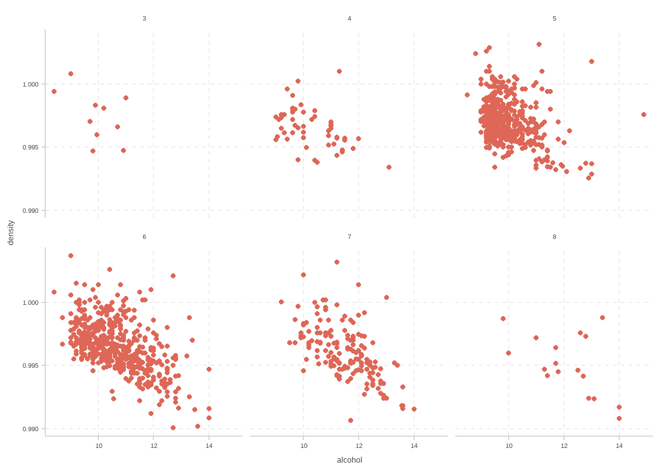
# 回归
```{r}
d <- read.csv("C:/Users/10156/Desktop/non/data/winequality-red.csv", sep=";")
ggplot(d)+
  geom_point(mapping=aes(x=alcohol,y=density))+
  facet_wrap(~quality)
```
## 样条光滑
$$
Y = \sum_{j=1}^p f_j(x_j) + \varepsilon
$$
$$
\begin{align}
\min_{f(\cdot)}
\left\{
\sum_i [y_i - f(x_i)]^2 + \lambda \int [f''(x)]^2 \,dx
\right\}
\end{align}
$$
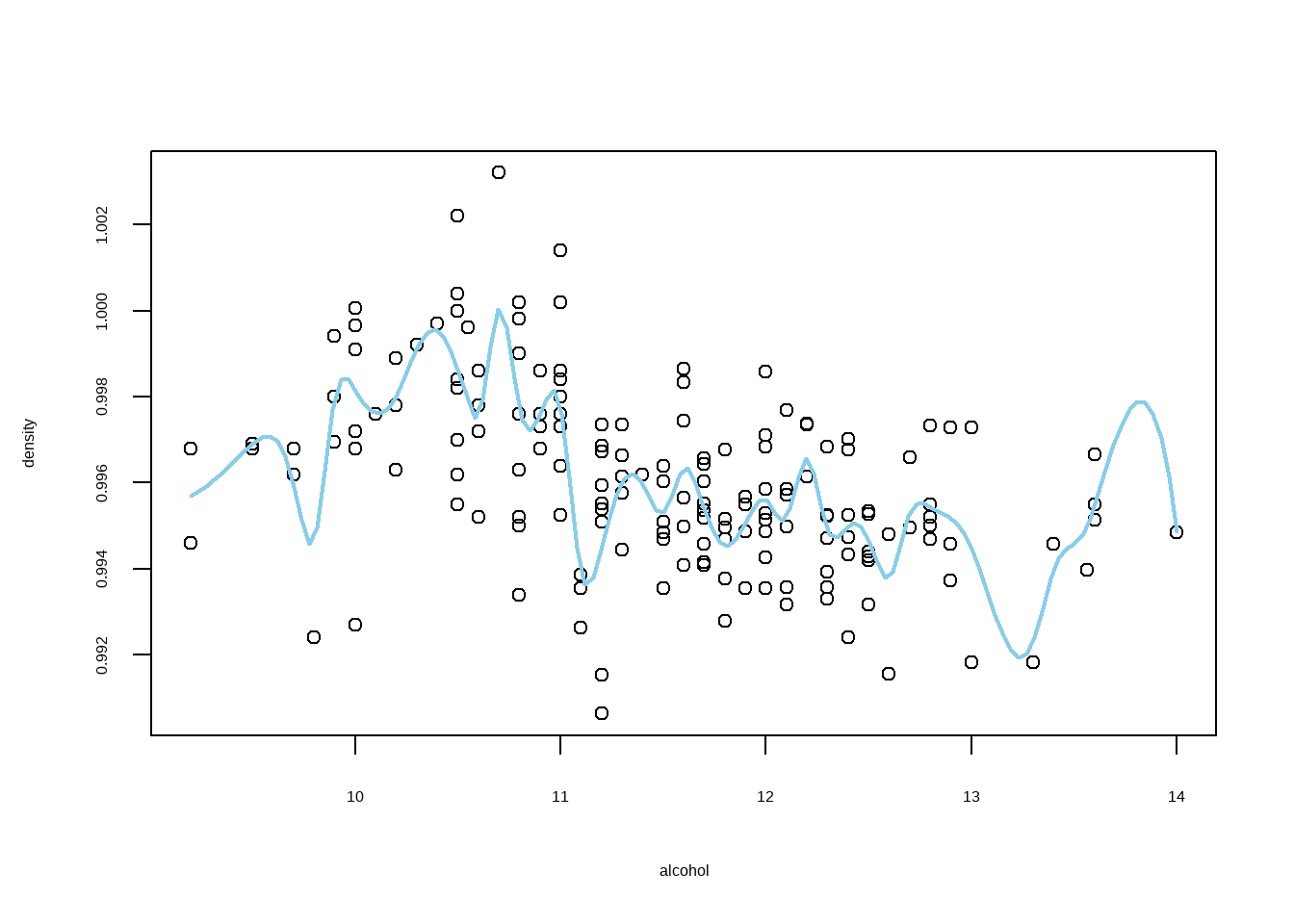
对质量7的红酒酒精浓度与酒密度进行样条光滑回归
```{r}
nsamp <- 53
alcohol <- (d %>% filter(quality==7))$alcohol
density <- (d %>% filter(quality==7))$density
alcohol=sort(alcohol)
plot(alcohol,density)
library(splines)
res <- smooth.spline(alcohol, density)
lines(spline(res$x, res$y), col="skyblue",lwd=2)
```
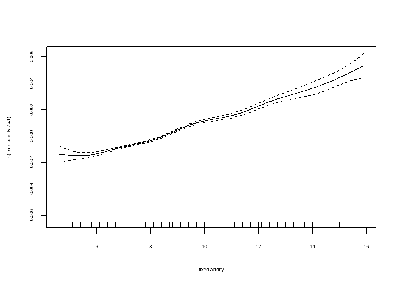
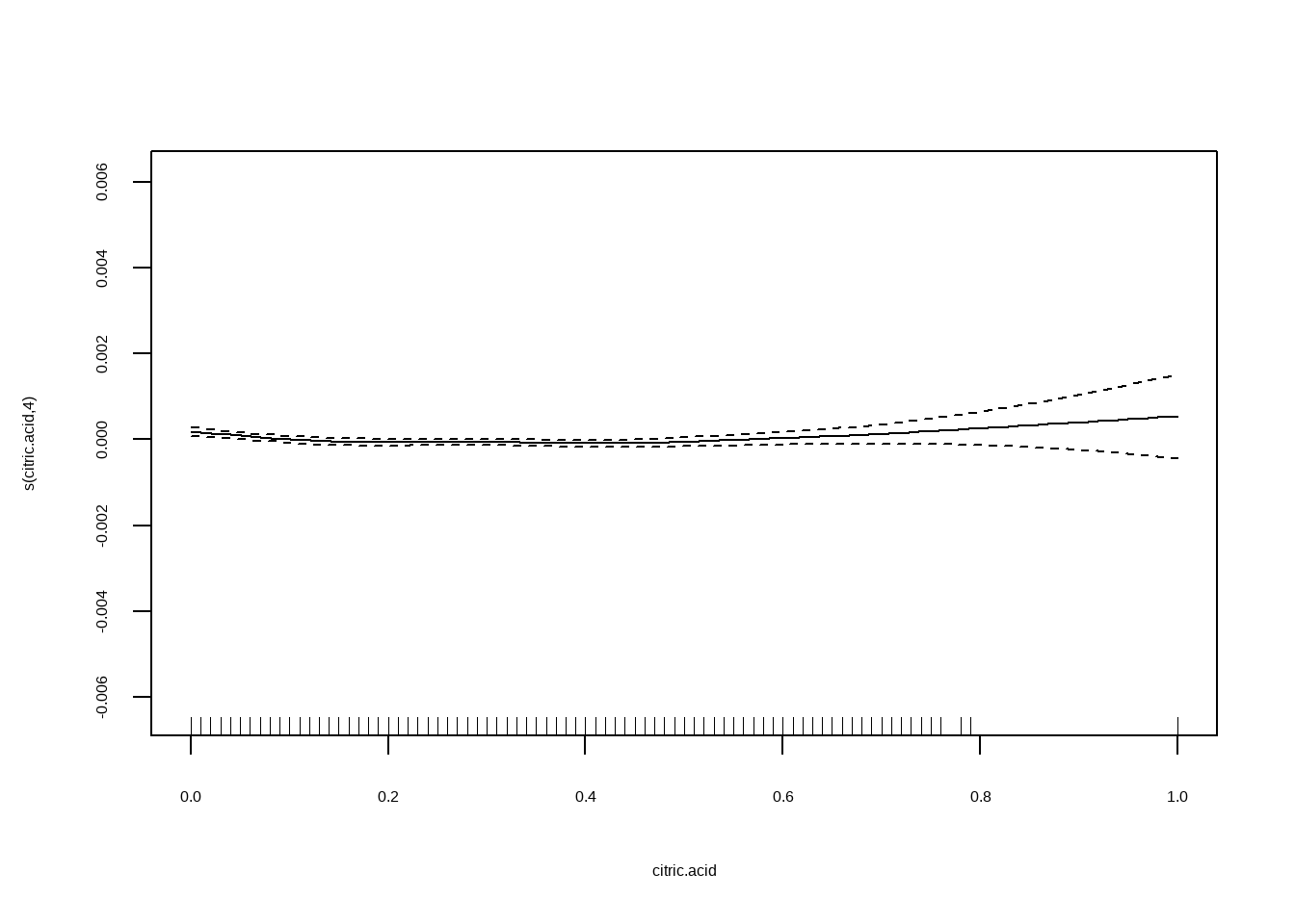
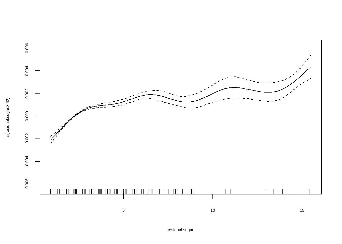
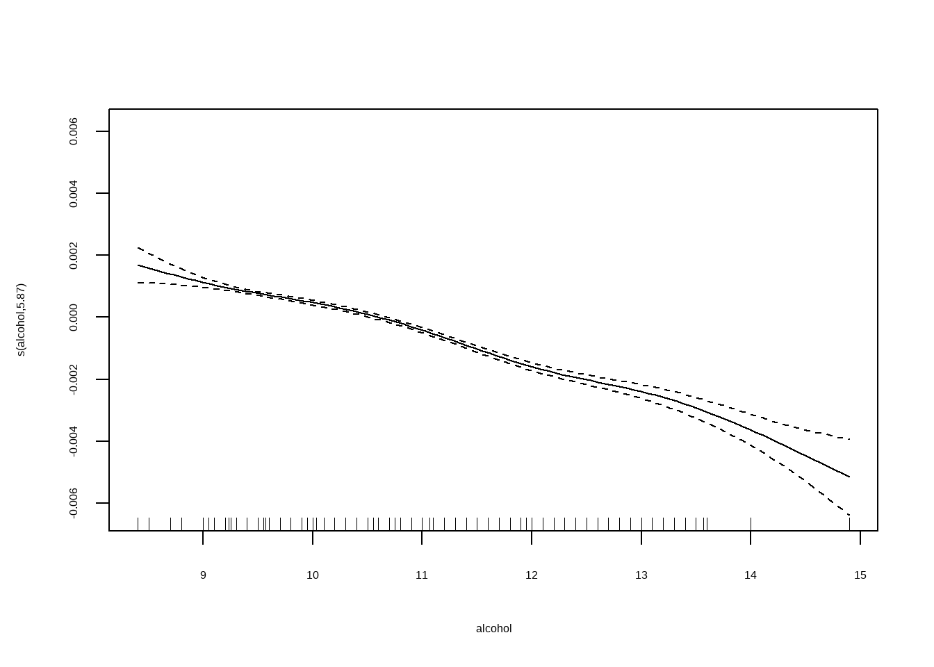
## Generalized Additive Model (GAM)线性可加模型
将`density`作为因变量,自变量为`fixed.acidity, citric.acid, residual.sugar与alcohol`
```{r}
library(mgcv)

fit2 <- gam(
  log(density) ~ s(fixed.acidity) + s(citric.acid) + s(residual.sugar)+s(alcohol), data=d)
summary(fit2)
```
```{r}
plot(fit2)
```