---
title: R包tidymodels
author: 'Kili'
date: "2024-08-02"
categories: ["R","tidymodels","机器学习"]
image: tidymodels.png
toc: true
cache: true
---
载入R包:
```{r}
library(tidymodels) # for the parsnip package, along with the rest of tidymodels

# Helper packages
library(readr) # for importing data
library(broom.mixed) # for converting bayesian models to tidy tibbles
library(dotwhisker) # for visualizing regression results
```
```{r}
urchins <-
  read_csv("urchins.csv") %>%
  setNames(c("food_regime", "initial_volume", "width")) %>%
  mutate(food_regime = factor(food_regime, levels = c("Initial", "Low", "High")))

glimpse(urchins)
```
```{r}
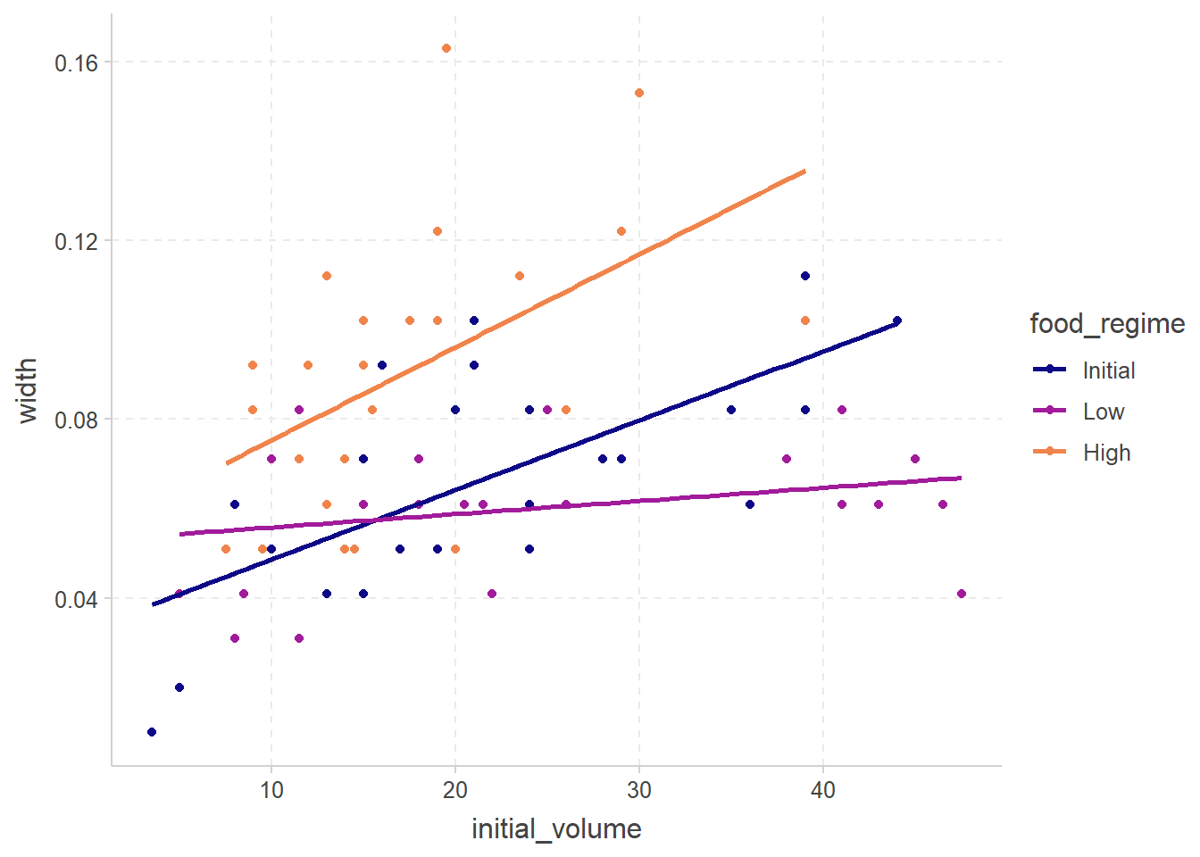
#| fig-cap: 按喂养食物进行分组线性回归
ggplot(
urchins,
aes(
x = initial_volume,
y = width,
group = food_regime,
col = food_regime
)
) +
geom_point() +
geom_smooth(method = lm, se = FALSE) +
scale_color_viridis_d(option = "plasma", end = .7)
```
进行线性回归可用的引擎:
```{r}
show_engines("linear_reg")
```
# 预处理数据--recipes
```{r}
library(tidymodels) # for the recipes package, along with the rest of tidymodels

# Helper packages
library(nycflights13) # for flight data
library(skimr) # for variable summaries
```
载入航班数据预测是否晚点
```{r}
set.seed(123)

flight_data <-
  flights %>%
  mutate(
    # Convert the arrival delay to a factor
    arr_delay = ifelse(arr_delay >= 30, "late", "on_time"),
    arr_delay = factor(arr_delay),
    # We will use the date (not date-time) in the recipe below
    date = lubridate::as_date(time_hour)
  ) %>%
  # Include the weather data
  inner_join(weather, by = c("origin", "time_hour")) %>%
  # Only retain the specific columns we will use
  select(
    dep_time, flight, origin, dest, air_time, distance,
    carrier, date, arr_delay, time_hour
  ) %>%
  # Exclude missing data
  na.omit() %>%
  # For creating models, it is better to have qualitative columns
  # encoded as factors (instead of character strings)
  mutate_if(is.character, as.factor)
```
看一眼:
```{r}
glimpse(flight_data)
```
其中flight与time_hour我们不希望将其作为预测数据,但保留为识别
## 划分训练与测试集
```{r}
# Fix the random numbers by setting the seed
# This enables the analysis to be reproducible when random numbers are used
set.seed(222)
# Put 3/4 of the data into the training set
data_split <- initial_split(flight_data, prop = 3 / 4)

# Create data frames for the two sets:
train_data <- training(data_split)
test_data <- testing(data_split)
```
## 开始创建食谱
```{r}
flights_rec <-
  recipe(arr_delay ~ ., data = train_data)
```
现在,我们可以向此配方添加角色。我们可以使用 update_role() 函数让食谱知道 flight 和 time_hour 是具有我们称为“ID”的自定义角色的变量(角色可以具有任何字符值)。虽然我们的公式将训练集中除 arr_delay 以外的所有变量都包括为预测因子,但这告诉配方保留这两个变量,但不要将它们用作结果或预测因子。
```{r}
flights_rec <-
  recipe(arr_delay ~ ., data = train_data) %>%
  update_role(flight, time_hour, new_role = "ID")
summary(flights_rec)
```
对日期进行特征工程
- 星期几,
- 月份,以及
- 该日期是否与假日相对应。
```{r}
flights_rec <-
  recipe(arr_delay ~ ., data = train_data) %>%
  update_role(flight, time_hour, new_role = "ID") %>%
  step_date(date, features = c("dow", "month")) %>%
  step_holiday(date,
    holidays = timeDate::listHolidays("US"), # us的假期
    keep_original_cols = FALSE
  ) %>%
  step_dummy(all_nominal_predictors()) %>%
  step_zv(all_predictors())
```
简单讲解一下: step_date与step_holiday用于对原日期进行转化,而keep_original_cols去除原日期,step_dummy(all_nominal_predictors())将所有nominal即名义变量转化为哑变量,step_zv去除数量过少的因子,例如
```{r}
test_data %>%
  distinct(dest) %>%
  anti_join(train_data)
```
dest中lex仅在test set有一个记录
```{r}
flights_rec[["var_info"]]$type
```
可见有四个变量被转化为了dummy变量
## 使用recipes
```{r}
lr_mod <-
  logistic_reg() %>%
  set_engine("glm")  # 设定引擎

flights_wflow <-
  workflow() %>%           # 创建工作流
  add_model(lr_mod) %>%    # 添加模型
  add_recipe(flights_rec)   # 添加食谱

flights_wflow  # 查看工作流
```
```{r}
flights_fit <-
  flights_wflow %>%
  fit(data = train_data)  # 拟合模型


flights_fit  # 查看模型


flights_fit %>%
  extract_fit_parsnip() %>%
  tidy()  # 查看模型参数

flights_fit %>%
  extract_recipe() %>%
  tidy()   # 查看食谱
```
# 建立线性回归model
用`fit()`函数
```{r}
linear_reg() %>%
  set_engine("keras") # 设定引擎
```
```{r}
lm_mod <- linear_reg() # 保存
lm_fit <-
  lm_mod %>%
  fit(width ~ initial_volume * food_regime, data = urchins)
lm_fit
```
查看一下lm_fit的属性,与传统`lm()`函数进行对比
```{r}
attributes(lm_fit)
attributes(lm_fit$fit)
lm(width ~ initial_volume * food_regime, data = urchins) |> attributes()
```
tidy一下
```{r}
tidy(lm_fit)
```
# 预测
```{r}
new_points <- expand.grid(
  initial_volume = 20,
  food_regime = c("Initial", "Low", "High")
)
new_points
```
预测一下初始体积20下的最终大小
```{r}
mean_pred <- predict(lm_fit, new_data = new_points)
mean_pred
conf_int_pred <- predict(lm_fit,
  new_data = new_points,
  type = "conf_int"
)
conf_int_pred
```
# 非线性
先导入数据
```{r}
library(tidymodels)
library(ISLR)

Wage <- as_tibble(Wage)
```
## 多项式回归与step functions
`step_poly(age, degree = 4)`将age进行4次多项式转化
```{r}
rec_poly <- recipe(wage ~ age, data = Wage) %>%
  step_poly(age, degree = 4)

lm_spec <- linear_reg() %>%
  set_mode("regression") %>%
  set_engine("lm")

poly_wf <- workflow() %>%
  add_model(lm_spec) %>%
  add_recipe(rec_poly)

poly_fit <- fit(poly_wf, data = Wage)
poly_fit
```
```{r}
tidy(poly_fit)
```
事实上step_poly()并没有返回age、age^2、age^3和age^4,它返回的变量是正交多项式的基,这意味着每一列都是变量age、age ^2、age ^3和age ^4的线性组合。
```{r}
q <- poly(1:6, degree = 4, raw = FALSE)
q
poly(1:6, degree = 4, raw = TRUE)
round(sum(q[, 1] * q[, 2]))
```
已经施密特正交化以减少共线性
如果想用原数据:
```
rec_raw_poly <- recipe(wage ~ age, data = Wage) %>%
  step_poly(age, degree = 4, options = list(raw = TRUE))

raw_poly_wf <- workflow() %>%
  add_model(lm_spec) %>%
  add_recipe(rec_raw_poly)

raw_poly_fit <- fit(raw_poly_wf, data = Wage)

tidy(raw_poly_fit)
```
now,用`poly_fit`来拟合一些数据
```{r}
age_range <- tibble(age = seq(min(Wage$age), max(Wage$age)))

regression_lines <- bind_cols(
  augment(poly_fit, new_data = age_range),
  predict(poly_fit, new_data = age_range, type = "conf_int")
)
regression_lines
```
```{r}
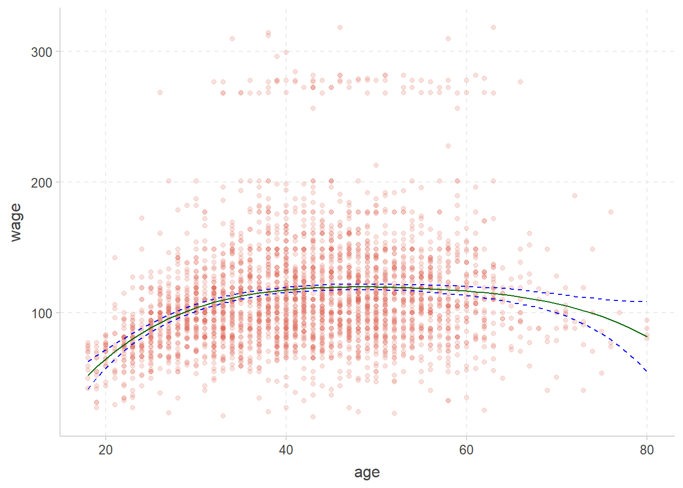
#| fig-cap: 绿色为回归,蓝色为置信区间
Wage %>%
ggplot(aes(age, wage)) +
geom_point(alpha = 0.2) +
geom_line(aes(y = .pred),
color = "darkgreen",
data = regression_lines
) +
geom_line(aes(y = .pred_lower),
data = regression_lines,
linetype = "dashed", color = "blue"
) +
geom_line(aes(y = .pred_upper),
data = regression_lines,
linetype = "dashed", color = "blue"
)
```
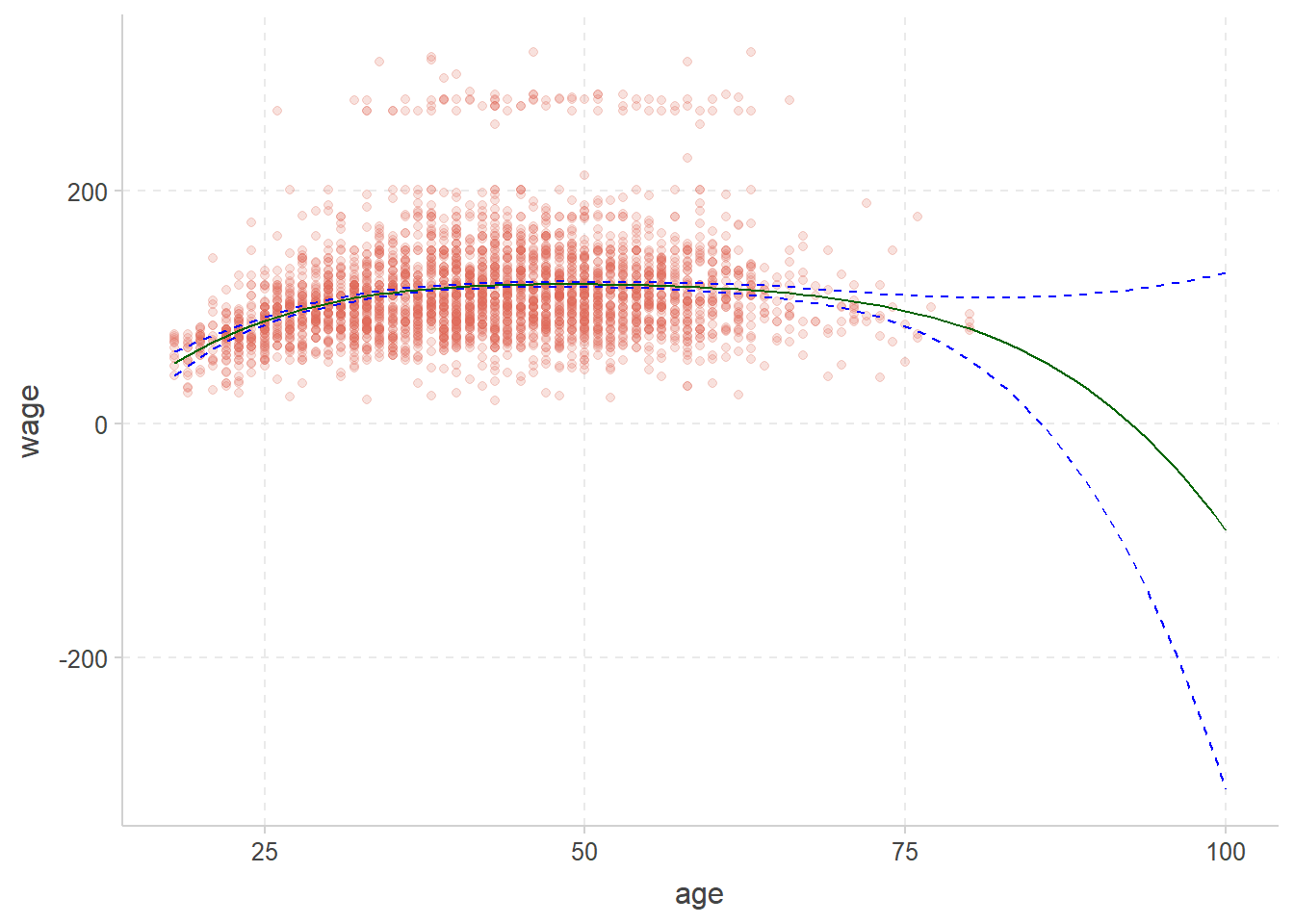
现在预测更大的年龄范围(18~100)
```{r}
wide_age_range <- tibble(age = seq(18, 100))
regression_lines <- bind_cols(
augment(poly_fit, new_data = wide_age_range),
predict(poly_fit, new_data = wide_age_range, type = "conf_int")
)
Wage %>%
ggplot(aes(age, wage)) +
geom_point(alpha = 0.2) +
geom_line(aes(y = .pred),
color = "darkgreen",
data = regression_lines
) +
geom_line(aes(y = .pred_lower),
data = regression_lines,
linetype = "dashed", color = "blue"
) +
geom_line(aes(y = .pred_upper),
data = regression_lines,
linetype = "dashed", color = "blue"
)
```
边缘处的置信区间变得更大,方差过大,model预测效果不好.
# 参考
- [李东风R语言教程](https://www.math.pku.edu.cn/teachers/lidf/docs/Rbook/html/_Rbook/stat-tidy-basic.html)
- [ISLR ISLR (英语)](https://emilhvitfeldt.github.io/ISLR-tidymodels-labs/)
- [tidymodels 整洁的模型](https://www.tidymodels.org/start/models/)