Code
```{r}
#| label: setup
library(ggplot2)
library(tidyverse)
library(tidymodels)
library(haven)
d <- read_dta("data/nsw_cps.dta")

d <- d |> mutate(across(\(col) length(unique(col))<3, as.factor))
```最近在做因果推断作业时遇到一个有趣的问题:
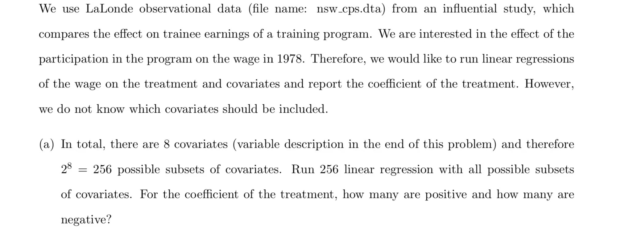
即以re78为outcome,treat 为treatment,其他八个变量为covariate进行256次建立model,毫无疑问这需要函数编程与向量化.
here’s the data:data/nsw_cps.dta
```{r}
#| label: setup
library(ggplot2)
library(tidyverse)
library(tidymodels)
library(haven)
d <- read_dta("data/nsw_cps.dta")
d <- d |> mutate(across(\(col) length(unique(col))<3, as.factor))
```看一眼
```{r}
glimpse(d)
```
Rows: 2,554
Columns: 11
$ data_id <fct> CPS2, CPS2, CPS2, CPS2, CPS2, CPS2, CPS2, CPS2, CPS2, CPS2, …
$ treat <fct> 0, 0, 0, 0, 0, 0, 0, 0, 0, 0, 0, 0, 0, 0, 0, 0, 0, 0, 0, 0, …
$ age <dbl> 16, 16, 16, 16, 16, 16, 16, 16, 16, 16, 16, 16, 16, 16, 16, …
$ education <dbl> 1, 6, 6, 7, 7, 7, 7, 8, 8, 8, 8, 8, 8, 8, 8, 8, 8, 8, 8, 8, …
$ black <fct> 0, 0, 1, 0, 0, 0, 1, 0, 0, 0, 0, 0, 0, 0, 0, 0, 0, 0, 0, 0, …
$ hispanic <fct> 0, 1, 0, 0, 0, 1, 0, 0, 0, 0, 0, 0, 0, 0, 0, 0, 0, 0, 0, 0, …
$ married <fct> 0, 0, 0, 0, 0, 0, 0, 0, 0, 0, 0, 0, 0, 0, 0, 0, 0, 0, 0, 0, …
$ nodegree <fct> 1, 1, 1, 1, 1, 1, 1, 1, 1, 1, 1, 1, 1, 1, 1, 1, 1, 1, 1, 1, …
$ re74 <dbl> 0.0000, 164.5784, 0.0000, 0.0000, 658.3136, 289.9715, 133.23…
$ re75 <dbl> 930.96771, 35.80645, 44.75806, 975.72583, 479.80649, 0.00000…
$ re78 <dbl> 2351.0630, 1640.2760, 0.0000, 4728.7251, 6210.8848, 7515.716…先用makeFormulae函数创建256个公式对象,fomula对象是一个list
```{r}
library(statisfactory)
fomula <- makeFormulae(re78 ~ age + education + black + hispanic + married + nodegree + re74 + re75, quad = F, ia = F)
fomula <- map(fomula,update,.~.+treat)
length(fomula)
head(fomula)
```
[1] 256
[[1]]
re78 ~ age + treat
<environment: 0x0000000023461340>
[[2]]
re78 ~ education + treat
<environment: 0x0000000023461340>
[[3]]
re78 ~ black + treat
<environment: 0x0000000023461340>
[[4]]
re78 ~ hispanic + treat
<environment: 0x0000000023461340>
[[5]]
re78 ~ married + treat
<environment: 0x0000000023461340>
[[6]]
re78 ~ nodegree + treat
<environment: 0x0000000023461340>接着创建256个工作流程(具体看tidymodels的官网)
```{r}
lm_mod <- linear_reg()

models <-
  workflow_set(preproc = fomula,models= list(lm_mod))

head(models)
```
# A workflow set/tibble: 6 × 4
wflow_id info option result
<chr> <list> <list> <list>
1 formula_1_linear_reg <tibble [1 × 4]> <opts[0]> <list [0]>
2 formula_2_linear_reg <tibble [1 × 4]> <opts[0]> <list [0]>
3 formula_3_linear_reg <tibble [1 × 4]> <opts[0]> <list [0]>
4 formula_4_linear_reg <tibble [1 × 4]> <opts[0]> <list [0]>
5 formula_5_linear_reg <tibble [1 × 4]> <opts[0]> <list [0]>
6 formula_6_linear_reg <tibble [1 × 4]> <opts[0]> <list [0]>为每个公式创建具体模型拟合,保存至fit列,至此我们便做了256此回归,得到256个lm对象(储存在fit列)
```{r}
models <-
  models |>
  mutate(fit = map(info,~ fit(.x$workflow[[1]],d)))
head(tidy(models$fit[[1]]))
```
# A tibble: 3 × 5
term estimate std.error statistic p.value
<chr> <dbl> <dbl> <dbl> <dbl>
1 (Intercept) 6061. 458. 13.2 1.02e-38
2 age 145. 14.9 9.74 5.13e-22
3 treat1 -3467. 660. -5.26 1.59e- 7```{r}
fit <- models$fit
fit[[1]]
tidy_fit <- map(fit,tidy)
tidy_fit[[1]]
```══ Workflow [trained] ══════════════════════════════════════════════════════════
Preprocessor: Formula
Model: linear_reg()
── Preprocessor ────────────────────────────────────────────────────────────────
re78 ~ age + treat
── Model ───────────────────────────────────────────────────────────────────────
Call:
stats::lm(formula = ..y ~ ., data = data)
Coefficients:
(Intercept) age treat1
6060.6 145.5 -3467.2
# A tibble: 3 × 5
  term        estimate std.error statistic  p.value
  <chr>          <dbl>     <dbl>     <dbl>    <dbl>
1 (Intercept)    6061.     458.      13.2  1.02e-38
2 age             145.      14.9      9.74 5.13e-22
3 treat1 -3467. 660. -5.26 1.59e- 7不妨再统计一下不同线性回归模型treat的系数与统计显著性
```{r}
q <- map(tidy_fit,~filter(.x,term=="treat1"))
head(q)
q1 <- q |> map_dbl(2)
q2 <- q |> map_dbl(5)
```
[[1]]
# A tibble: 1 × 5
term estimate std.error statistic p.value
<chr> <dbl> <dbl> <dbl> <dbl>
1 treat1 -3467. 660. -5.26 0.000000159
[[2]]
# A tibble: 1 × 5
term estimate std.error statistic p.value
<chr> <dbl> <dbl> <dbl> <dbl>
1 treat1 -3301. 664. -4.97 0.000000703
[[3]]
# A tibble: 1 × 5
term estimate std.error statistic p.value
<chr> <dbl> <dbl> <dbl> <dbl>
1 treat1 -2009. 777. -2.59 0.00975
[[4]]
# A tibble: 1 × 5
term estimate std.error statistic p.value
<chr> <dbl> <dbl> <dbl> <dbl>
1 treat1 -3846. 671. -5.73 0.0000000109
[[5]]
# A tibble: 1 × 5
term estimate std.error statistic p.value
<chr> <dbl> <dbl> <dbl> <dbl>
1 treat1 -2646. 657. -4.03 0.0000583
[[6]]
# A tibble: 1 × 5
term estimate std.error statistic p.value
<chr> <dbl> <dbl> <dbl> <dbl>
1 treat1 -3020. 666. -4.53 0.00000611```{r}
dd <- tibble(coef=q1,p=q2)
head(dd)
dd |> summarise(positive=sum(coef>0),
negative=sum(coef<0),
posi_sign=sum(coef>0 & p<0.05),
posi_nosign=sum(coef>0 & p>0.05),
nega_sign=sum(coef<0 & p<0.05),
nega_nosign=sum(coef<0&p>0.05))
```# A tibble: 6 × 2
coef p
<dbl> <dbl>
1 -3467. 0.000000159
2 -3301. 0.000000703
3 -2009. 0.00975
4 -3846. 0.0000000109
5 -2646. 0.0000583
6 -3020. 0.00000611
# A tibble: 1 × 6
positive negative posi_sign posi_nosign nega_sign nega_nosign
<int> <int> <int> <int> <int> <int>
1 148 108 3 145 39 69