---
title: |
Survival analysis of \
Skin Cutaneous Melanoma[SKCM]
subtitle: A case study of The Cancer Genome Atlas,TCGA
author: 'Kili'
date: "2024-08-14"
thanks: personal blog:<https://sysukili.netlify.app/>
abstract: >
癌症基因组图谱计划(The Cancer Genome,Atlas,TCGA)是美国的国家肿瘤研究所(National Cancer Institute,NCI)与国家人类基因研究所(National Human Genome Research Institute,NHGRI)共同开展的一个广泛而综合的合作计划。其目标是获取、刻画并分析人类癌症中大规模、多种变异的分子特征,且为癌症研究迅速地提供数据。选取发病于皮肤的皮肤黑色素瘤样本[SKCM],即Skin Cutaneous Melanoma作为生存分析对象.分析不同样本特征下的死亡率差别.
lang: zh
number-sections: true
crossref:
chapters: true
execute:
warning: false
cache: true
---
\newpage
```{r}
library(survival)
library(survminer)
library(autoReg)
library(readr)
library(survMisc)
library(easystats)
library(tidyverse)
library(gtsummary)
library(rms)
library(conflicted)
library(ggplot2)
library(scales)
conflicts_prefer(dplyr::filter)
conflicts_prefer(dplyr::summarize)
conflicts_prefer(dplyr::select)
skcm <- read_delim("data/skcm_new.csv",
  delim = "\t", escape_double = FALSE,
  col_types = cols(form_completion_date = col_date(format = "%Y-%m-%d"), birth_days_to = col_number()),
  trim_ws = TRUE
)
```
```{r}
sum_of_na <- function(x) {
  sum(is.na(x))
}
skcm %>% summarise(
  across(everything(), sum_of_na)
)
```
# 数据背景
Melanoma is a cancer in a type of skin cells called melanocytes. Melanocyes are the cells that produce melanin, which colors the skin. When exposed to sun, these cells make more melanin, causing the skin to darken or tan. Melanoma can occur anywhere on the body and risk factors include fair complexion, family history of melanoma, and being exposed to natural or artificial sunlight over long periods of time. Melanoma is most often discovered because it has metastasized, or spread, to another organ, such as the lymph nodes. In many cases, the primary skin melanoma site is never found. Because of this challenge, TCGA is studying primarily metastatic cases (in contrast to other cancers selected for study, where metastatic cases are excluded). For 2011, it was estimated that there were 70,230 new cases of melanoma and 8,790 deaths from the disease
# 数据清洗与数据预览
先预览数据:
```{r}
#| tbl-cap: 数据预览
skcm <- skcm |>
  select(!bcr_patient_barcode:bcr_patient_uuid) |>
  select(!submitted_tumor_dx_days_to)
skcm <- skcm |> dplyr::select(days, status, height_cm_at_diagnosis, weight_kg_at_diagnosis, breslow_thickness_at_diagnosis, primary_melanoma_mitotic_rate, age_at_diagnosis, prospective_collection, gender, tumor_status, clark_level_at_diagnosis, primary_melanoma_tumor_ulceration, ajcc_tumor_pathologic_pt, ajcc_nodes_pathologic_pn, submitted_tumor_site.1, radiation_treatment_adjuvant, new_tumor_event_dx_indicator)
skcm <- skcm %>%
  mutate(across(function(col) n_distinct(col) < 10, factor)) %>%
  as_tibble()

gtsummary::tbl_summary(skcm, by = "tumor_status") %>%
  as_flex_table() |>
  flextable::set_caption("Summary statistics.by~tumor_status") %>%
  flextable::theme_zebra()
```
显然这是右删失数据,status=1代表死亡,=2代表右删失
观察到有缺失值,进行删除与补全
```{r}
#| output: false
skcm <- skcm |>
  dplyr::filter(days > 0) |>
  filter(!(is.na(radiation_treatment_adjuvant) | is.na(new_tumor_event_dx_indicator) | is.na(submitted_tumor_site.1) | is.na(submitted_tumor_site.1) | is.na(ajcc_nodes_pathologic_pn))) |>
  filter(!is.na(tumor_status))
skcm <- skcm |> filter(!is.na(ajcc_tumor_pathologic_pt))
skcm$height_cm_at_diagnosis[is.na(skcm$height_cm_at_diagnosis)] <- mean(na.omit(skcm$height_cm_at_diagnosis))
skcm$weight_kg_at_diagnosis[is.na(skcm$weight_kg_at_diagnosis)] <- mean(na.omit(skcm$weight_kg_at_diagnosis))
skcm$breslow_thickness_at_diagnosis[is.na(skcm$breslow_thickness_at_diagnosis)] <- mean(na.omit(skcm$breslow_thickness_at_diagnosis))
library(mice)
tempData <- mice(skcm, m = 5, maxit = 50, seed = 500)
completedData <- complete(tempData, action = 5)
skcm <- complete(tempData, action = 5)
```
将高度除以重量创造新特征BMI:
```{r}
skcm <- skcm |>
  mutate(BMI = height_cm_at_diagnosis / weight_kg_at_diagnosis) |>
  select(-height_cm_at_diagnosis, -weight_kg_at_diagnosis)
```
```{r}
head(skcm)
gaze(skcm)
```
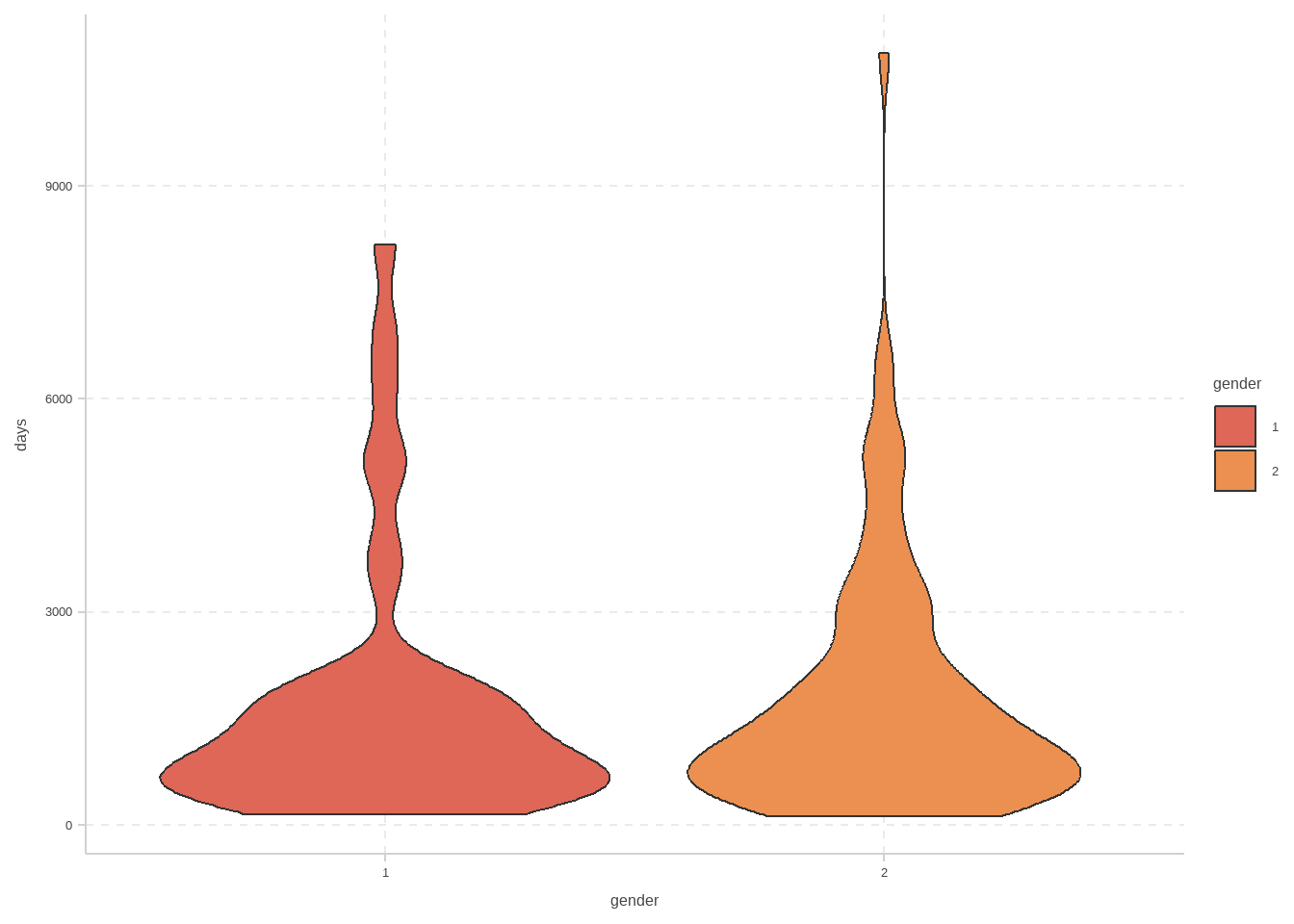
```{r}
#| fig-cap: 小提琴图
skcm |>
  filter(status == 1) |>
  ggplot(aes(x = gender, y = days, fill = gender)) +
  geom_violin()
```
# 预测模型
将数据集分为train与test:
```{r}
library(rsample)
set.seed(101)
skcm_split <- initial_split(
  skcm,
  prop = 0.90
)
train <- training(skcm_split)
test <- testing(skcm_split)
test.y <- test$class
```
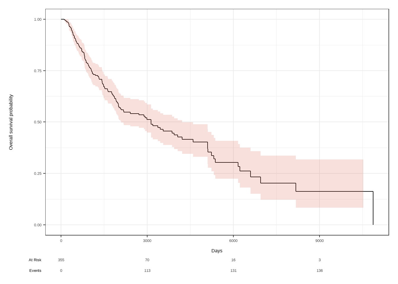
## Kaplan-Meier估计
```{r}
library(ggsurvfit)
library(tidycmprsk)
skcm$status <- as.numeric(skcm$status)
s <- Surv(skcm$days, skcm$status)
model1 <- survfit2(Surv(days, status) ~ 1, skcm)
model1 |> ggsurvfit() +
  labs(
    x = "Days",
    y = "Overall survival probability"
  ) +
  add_confidence_interval() +
  add_risktable()
```
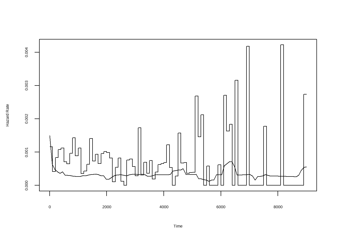
风险函数曲线估计与平滑化:
```{r}
library(muhaz)
result.pe1 <- pehaz(skcm$days, skcm$status, width = 100, max.time = 9000)
plot(result.pe1)
result.smooth <- muhaz(skcm$days, skcm$status,
  bw.smooth = 100,
  b.cor = "left", max.time = 9000
)
lines(result.smooth)
```
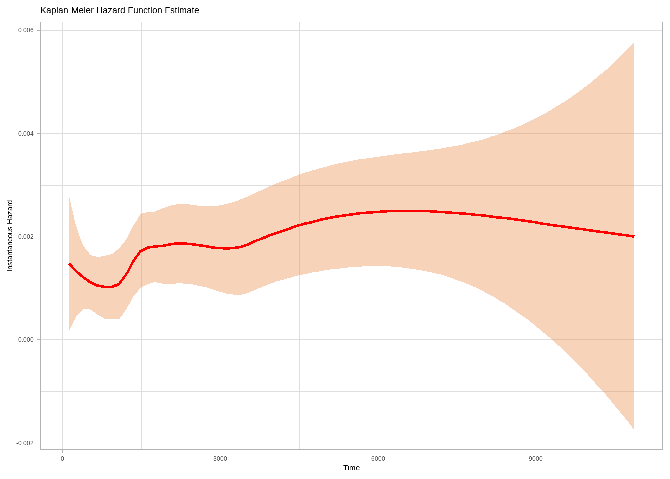
or:
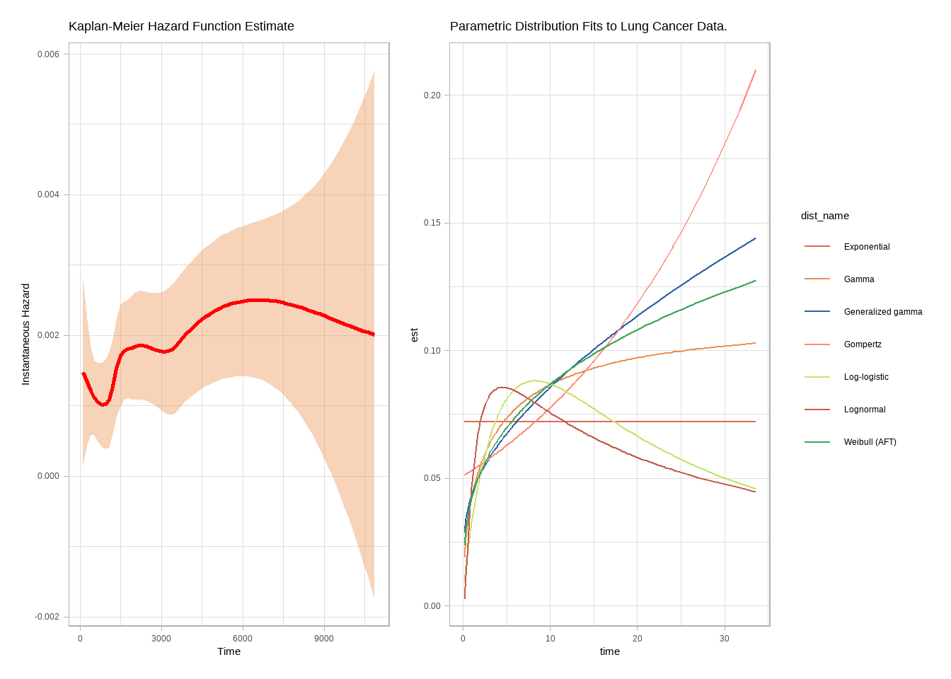
```{r}
p1 <- epiR::epi.insthaz(model1) %>%
  ggplot(aes(x = time, y = hest)) +
  geom_smooth(color = "red", method = "loess", formula = "y ~ x") +
  theme_light() +
  labs(
    title = "Kaplan-Meier Hazard Function Estimate",
    x = "Time", y = "Instantaneous Hazard"
  )
p1
```
## log-rank test
```{r}
survdiff(Surv(days, status) ~ strata(gender) + clark_level_at_diagnosis, data = skcm)
```
p值小,which is statistically significant at the 5 % level.
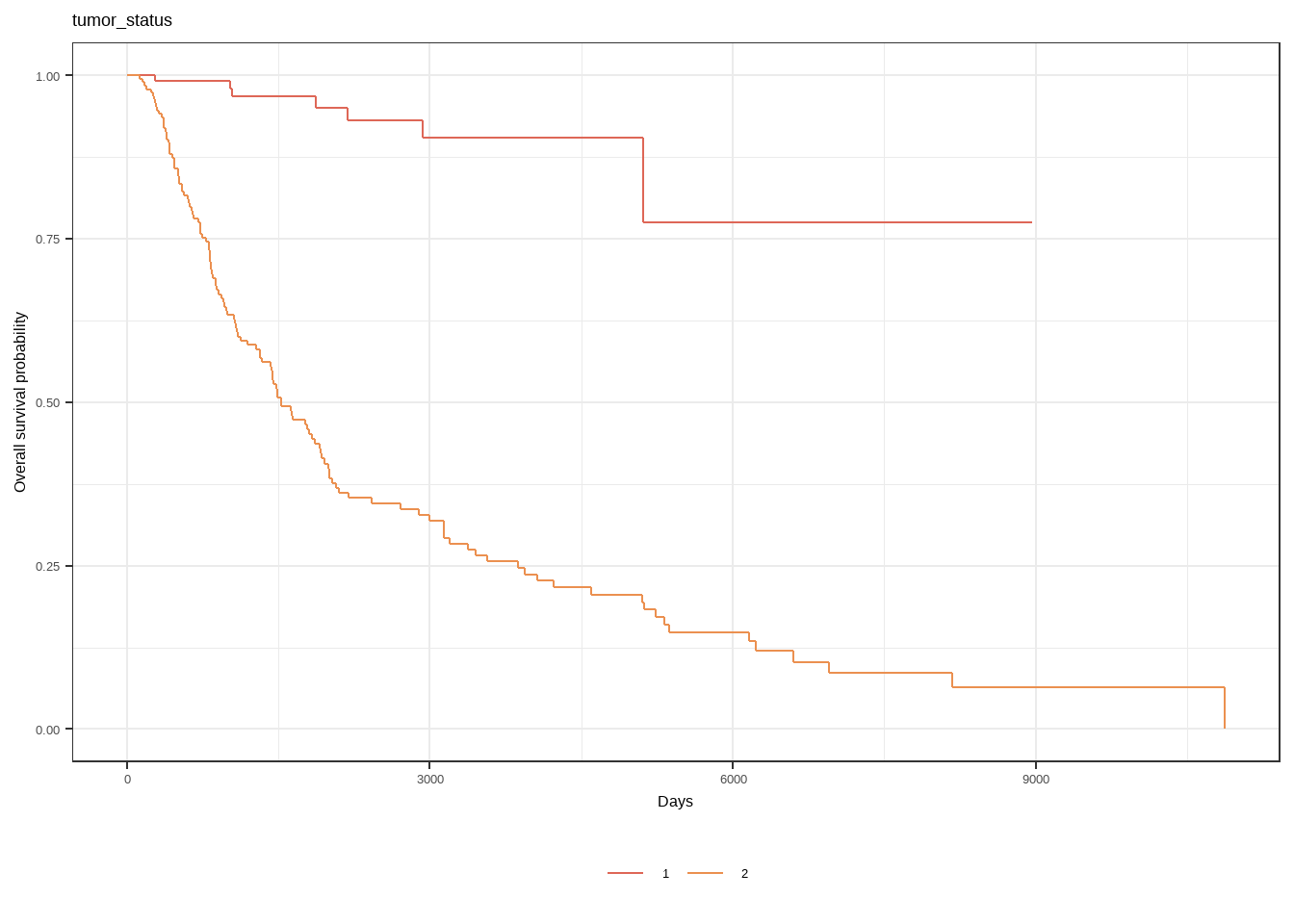
```{r}
library(ggsurvfit)
library(tidycmprsk)
skcm$status <- as.numeric(skcm$status)
s <- Surv(skcm$days, skcm$status)
model1 <- survfit2(Surv(days, status) ~ tumor_status, skcm)
model1 |> ggsurvfit() +
  labs(
    x = "Days",
    y = "Overall survival probability"
  ) + labs(title = "tumor_status")
```
## parametric mdoel
```{r}
library(flexsurv)
par_fits <- tibble(
  dist_param = c(
    "exp", "weibull", "gompertz", "gamma", "lognormal", "llogis",
    "gengamma"
  ),
  dist_name = c(
    "Exponential", "Weibull (AFT)", "Gompertz", "Gamma",
    "Lognormal", "Log-logistic", "Generalized gamma"
  )
) %>%
  mutate(
    fit = map(dist_param, ~ flexsurvreg(Surv(time, status) ~ 1, data = df_lung, dist = .x)),
    fit_smry = map(fit, ~ summary(.x, type = "hazard", ci = FALSE, tidy = TRUE)),
    AIC = map_dbl(fit, ~ .x$AIC)
  )

p2 <- par_fits %>%
  select(-c(dist_param, fit)) %>%
  unnest(fit_smry) %>%
  ggplot(aes(x = time, y = est, color = dist_name)) +
  geom_line() +
  theme_light() +
  labs(title = "Parametric Distribution Fits to Lung Cancer Data.")

p1 + p2
```
```{r}
par_fits %>%
  arrange(AIC) %>%
  select(dist_name, AIC)
```
比较AIC,最好的是Weibullmodel
```{r}
weibull_fit <- flexsurvreg(Surv(days, status) ~ age_at_diagnosis + tumor_status + clark_level_at_diagnosis + submitted_tumor_site.1, data = skcm, dist = "weibull")
weibull_fit
```
```{r}
new_dat <- expand.grid(
  age_at_diagnosis = median(skcm$age_at_diagnosis),
  tumor_status = levels(skcm$tumor_status),
  clark_level_at_diagnosis = levels(skcm$clark_level_at_diagnosis), submitted_tumor_site.1 = levels(skcm$submitted_tumor_site.1)
)
pre_weibull <- weibull_fit |> predict(type = "quantile", p = 0.5, newdata = new_dat)
head(bind_cols(pre_weibull, new_dat))
```
## 建立cox regression model
### the proportional hazards assumption
$$
h_1(t)=\psi h_0(t)
$$
```{r}
cox_fit <- coxph(Surv(days, status) ~ ., data = skcm)
cox_fit
(cox_tbl <- cox_fit %>% gtsummary::tbl_regression(exponentiate = TRUE, ))
```
故从age_at_diagnosis,tumor_status与submitted_tumor_site.1开始创建model
```{r}
cox_fit1 <- coxph(Surv(days, status) ~ age_at_diagnosis, data = skcm)
cox_fit2 <- coxph(Surv(days, status) ~ tumor_status, data = skcm)
cox_fit3 <- coxph(Surv(days, status) ~ submitted_tumor_site.1, data = skcm)
cox_fit1
cox_fit2
cox_fit3
```
由p值大小先将tumor_status加入model
逐步AIC确定最终model:
```{r}
result <- step(cox_fit, scope = list(upper = ~., lower = ~tumor_status))
```
```{r}
result
```
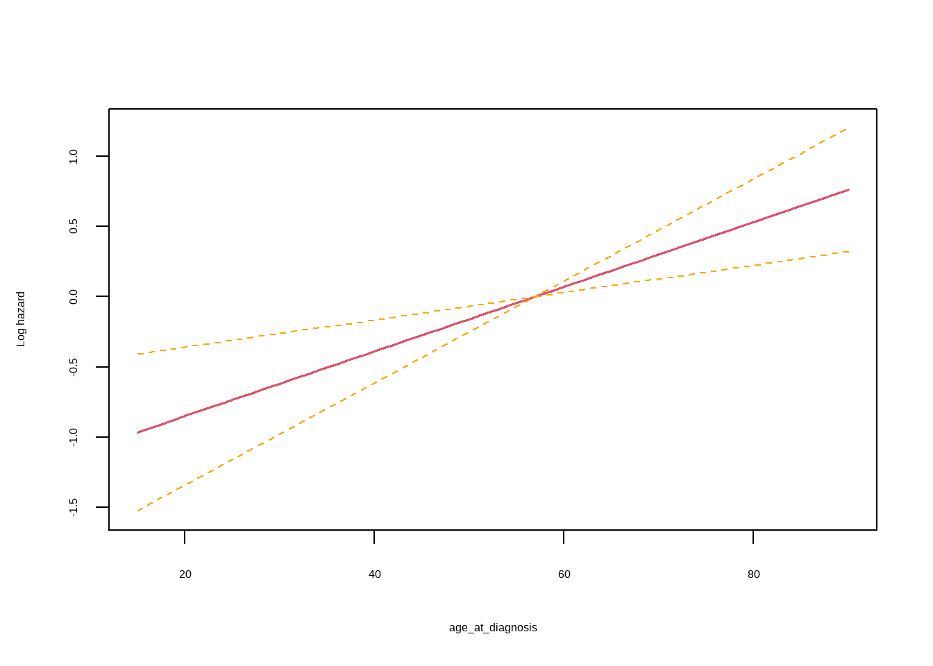
```{r}
termplot(result, se = T, terms = 1, ylabs = "Log hazard")
```
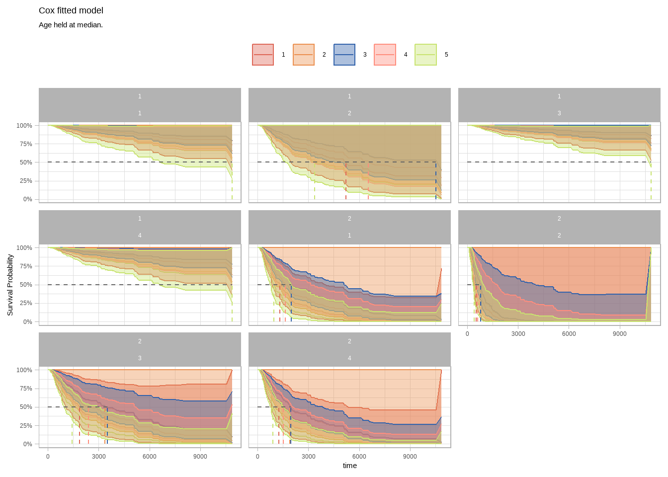
```{r}
cox_fit <- result
# Predictions will be for all levels of sex and ph.ecog, but only at the median
# age.
new_dat <- expand.grid(
  age_at_diagnosis = median(skcm$age_at_diagnosis),
  tumor_status = levels(skcm$tumor_status),
  clark_level_at_diagnosis = levels(skcm$clark_level_at_diagnosis), submitted_tumor_site.1 = levels(skcm$submitted_tumor_site.1)
) %>%
  # strata is our key to join back to the fitted values.
  mutate(strata = as.factor(row_number()))

# Create fitted survival curves at the covariate presets.
fit_curves <- survfit(cox_fit, newdata = new_dat, data = skcm)

# `surv_summary()` is like `summary()` except that it includes risk table info,
# confidence interval attributes, and pivots the strata longer.
surv_summary <- surv_summary(fit_curves) %>%
  # The cases are labeled "strata", but `survsummary()` doesn't label what the
  # strata are! Get it from new_dat.
  inner_join(new_dat, by = "strata")

# Now use ggplot() just like normal.
median_line <- surv_summary %>%
  filter(surv >= .5) %>%
  group_by(tumor_status, clark_level_at_diagnosis, submitted_tumor_site.1) %>%
  summarize(.groups = "drop", max_t = max(time))
surv_summary %>%
  ggplot(aes(x = time, y = surv)) +
  geom_line(aes(color = clark_level_at_diagnosis)) +
  geom_ribbon(aes(ymin = lower, ymax = upper, color = clark_level_at_diagnosis, fill = clark_level_at_diagnosis),
    alpha = 0.4
  ) +
  geom_segment(
    data = median_line,
    aes(x = 0, xend = max_t, y = .5, yend = .5),
    linetype = 2, color = "gray40"
  ) +
  geom_segment(
    data = median_line,
    aes(x = max_t, xend = max_t, y = 0, yend = .5, color = clark_level_at_diagnosis),
    linetype = 2
  ) +
  facet_wrap(facets = vars(tumor_status, submitted_tumor_site.1)) +
  scale_y_continuous(labels = percent_format(1)) +
  theme_light() +
  theme(legend.position = "top") +
  labs(
    X = "days", y = "Survival Probability", color = NULL, fill = NULL,
    title = "Cox fitted model",
    subtitle = "Age held at median."
  )
```
gender 分1,2 submitted_tumor_site.1分1,2,3,4
# 模型验证
## Assessing Goodness of Fit Using Residuals
### Martingale and Deviance Residuals
```{r}
smoothSEcurve <- function(yy, xx) {
# use after a call to "plot"
# fit a lowess curve and 95% confidence interval curve
# make list of x values
xx.list <- min(xx) + ((0:100) / 100) * (max(xx) - min(xx))
# Then fit loess function through the points (xx, yy)
# at the listed values
yy.xx <- predict(loess(yy ~ xx),
se = T,
newdata = data.frame(xx = xx.list)
)
lines(yy.xx$fit ~ xx.list, lwd = 2)
lines(yy.xx$fit -
qt(0.975, yy.xx$df) * yy.xx$se.fit ~ xx.list, lty = 2)
lines(yy.xx$fit +
qt(0.975, yy.xx$df) * yy.xx$se.fit ~ xx.list, lty = 2)
}
skcm1 <- select(skcm, age_at_diagnosis, tumor_status, clark_level_at_diagnosis, submitted_tumor_site.1)
rr.final <- residuals(cox_fit, type = "martingale")
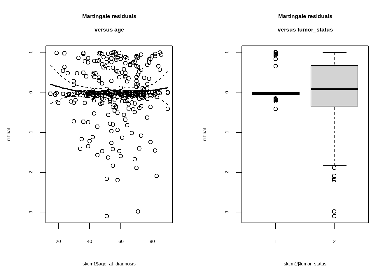
par(mfrow = c(1, 2))
plot(rr.final ~ skcm1$age_at_diagnosis)
smoothSEcurve(rr.final, skcm1$age_at_diagnosis)
title("Martingale residuals\nversus age")
plot(rr.final ~ skcm1$tumor_status)
title("Martingale residuals\nversus tumor_status")
```
```{r}
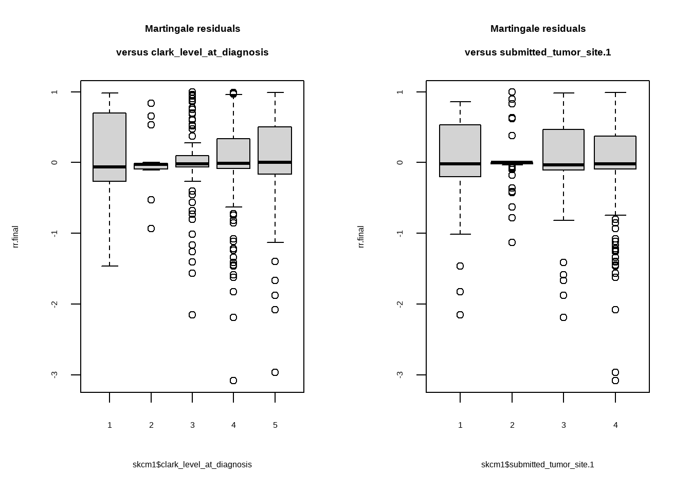
par(mfrow = c(1, 2))
plot(rr.final ~ skcm1$clark_level_at_diagnosis)
title("Martingale residuals\nversus clark_level_at_diagnosis")
plot(rr.final ~ skcm1$submitted_tumor_site.1)
title("Martingale residuals\nversus submitted_tumor_site.1")
```
残差大致均匀分布在0周围,可见model拟合效果不错
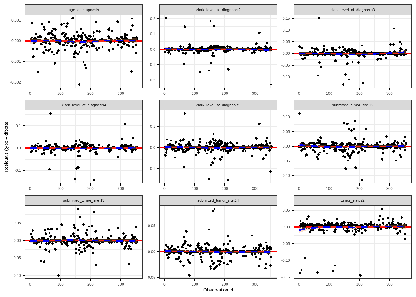
### Case Deletion Residuals
```{r}
ggcoxdiagnostics(cox_fit, type = "dfbeta", linear.predictions = FALSE)
```
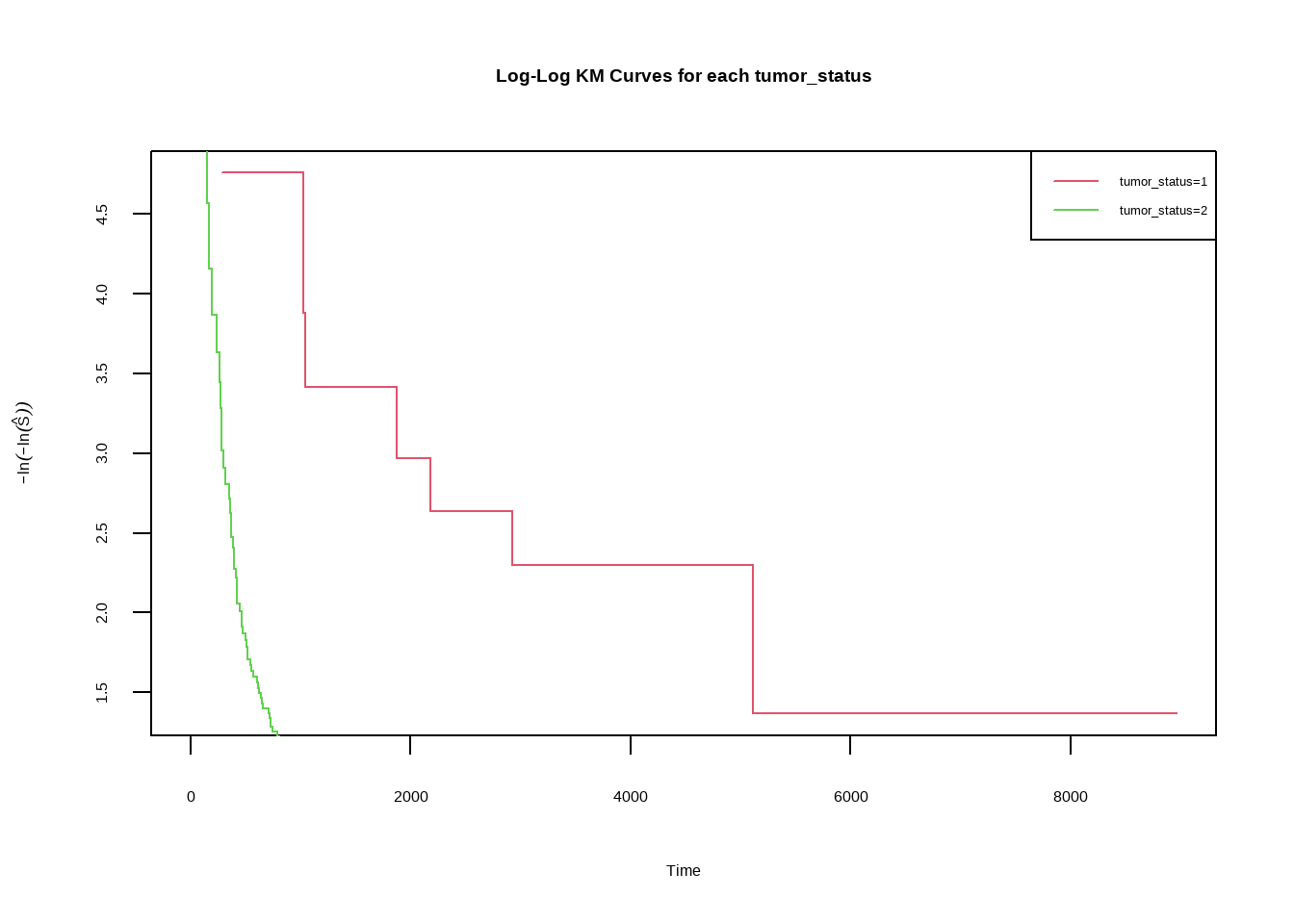
## Checking the Proportion Hazards Assumption
### Log Cumulative Hazard Plots
```{r}
fit <- survfit(Surv(days, status) ~ tumor_status, data = skcm)
fit$label <-
  c(rep(1, fit$strata[1]), rep(2, fit$strata[2]))
t1 <- c(0, subset(fit$time, fit$label == 1))
t2 <- c(0, subset(fit$time, fit$label == 2))

St1 <- c(1, subset(fit$surv, fit$label == 1))
St2 <- c(1, subset(fit$surv, fit$label == 2))
plot(t1, -log(-log(St1)), col = 2, type = "s", xlab = "Time", ylab = expression(-ln(-
  ln(hat(S)))), main = "Log-Log KM Curves for each tumor_status")

lines(t2, -log(-log(St2)), col = 3, type = "s")
legend("topright", c("tumor_status=1", "tumor_status=2"), col = 2:3, lty = 1, cex = 0.8)
```
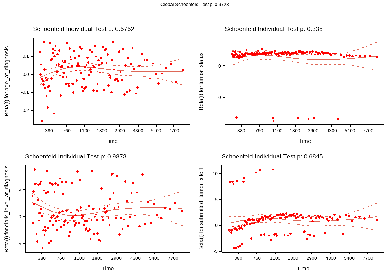
### Schoenfeld Residuals
```{r}
(cox_test_ph <- cox.zph(cox_fit))
ggcoxzph(cox_test_ph)
```
# 结果可视化
## ROC曲线
```{r}
train_model <- cox_fit
train <- skcm
library(timeROC)

train$lp <- predict(train_model, newdata = skcm1, type = "lp")
time_roc_train <- timeROC(
  T = train$days, # 结局时间
  delta = train$status, # 生存结局
  marker = train$lp, # 预测变量
  cause = 1, # 阳性结局指标值
  weighting = "marginal", # 权重计算方法,默认marginal,采用KM计算删失分布
  times = c(365, 730, 1100),
  ROC = TRUE, # 保存sensitivities 和 specificties值
  iid = TRUE # iid = TRUE 才会保存置信区间,但是样本量大了后,耗时耗资源
)

# 计算train-1年的AUC
train1y <- paste0(
  "train 1 year AUC (95%CI) = ",
  sprintf("%.3f", time_roc_train$AUC[1]), " (",
  sprintf("%.3f", confint(time_roc_train, level = 0.95)$CI_AUC[1, 1] / 100), " - ",
  sprintf("%.3f", confint(time_roc_train, level = 0.95)$CI_AUC[1, 2] / 100), ")"
)

# 计算train-3年的AUC
train3y <- paste0(
  "train 3 year AUC (95%CI) = ",
  sprintf("%.3f", time_roc_train$AUC[2]), " (",
  sprintf("%.3f", confint(time_roc_train, level = 0.95)$CI_AUC[2, 1] / 100), " - ",
  sprintf("%.3f", confint(time_roc_train, level = 0.95)$CI_AUC[2, 2] / 100), ")"
)

# 计算train-5年的AUC
train5y <- paste0(
  "train 5 year AUC (95%CI) = ",
  sprintf("%.3f", time_roc_train$AUC[3]), " (",
  sprintf("%.3f", confint(time_roc_train, level = 0.95)$CI_AUC[3, 1] / 100), " - ",
  sprintf("%.3f", confint(time_roc_train, level = 0.95)$CI_AUC[3, 2] / 100), ")"
)

# train AUC 多时间点合一
plot(title = "", time_roc_train, col = "DodgerBlue", time = 365, lty = 1, lwd = 2, family = "serif") # 绘制ROC曲线
plot(time_roc_train, time = 730, lty = 1, lwd = 2, add = TRUE, col = "LightSeaGreen", family = "serif") # add=TRUE指在前一条曲线基础上新增
plot(time_roc_train, time = 1100, lty = 1, lwd = 2, add = TRUE, col = "DarkOrange", family = "serif")
legend("bottomright", c(train1y, train3y, train5y), col = c("DodgerBlue", "LightSeaGreen", "DarkOrange"), lty = 1, lwd = 2)
```
效果不是很好😅
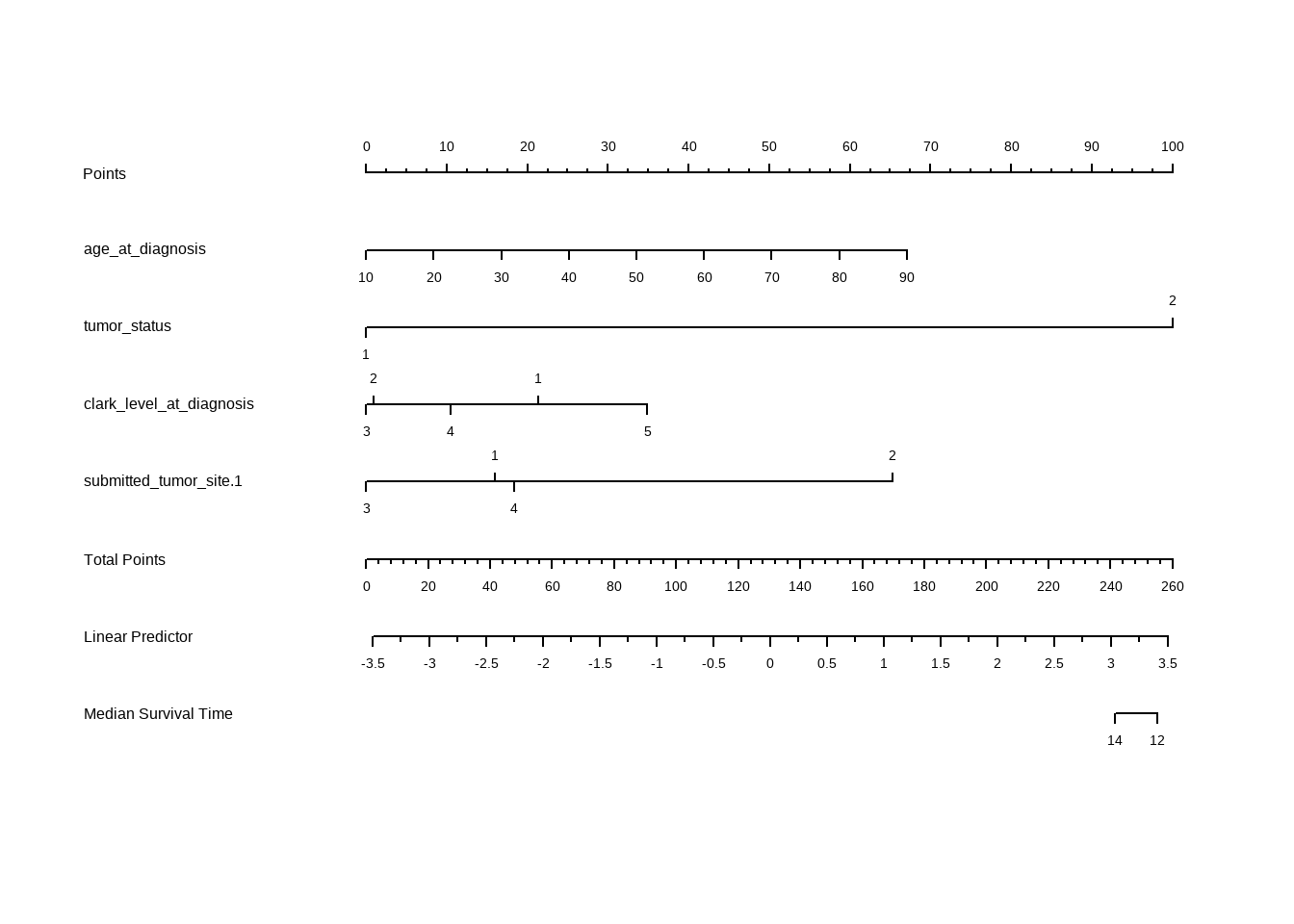
## nomogram
```{r}
skcm2 <- skcm |> mutate(months = floor(days / 30))
d <- datadist(skcm2)
options(datadist = "d")
f <- cph(formula = Surv(months, status) ~ age_at_diagnosis + tumor_status +
clark_level_at_diagnosis + submitted_tumor_site.1, data = skcm2, surv = T)
med <- Quantile(f)
surv <- Survival(f) # This would also work if f was from cph
plot(nomogram(f, fun = function(x) med(lp = x), funlabel = "Median Survival Time"))
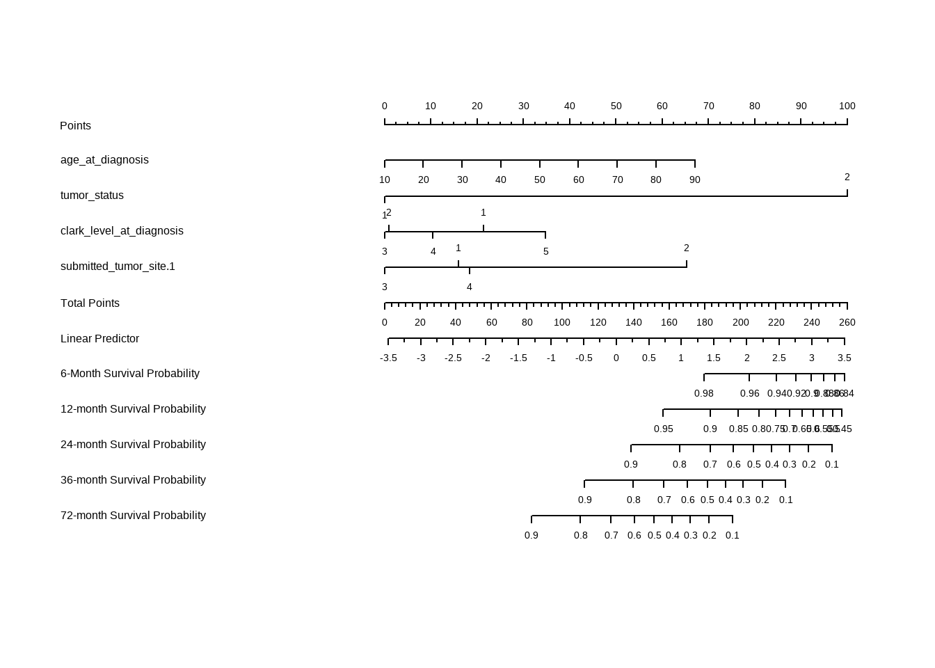
nom <- nomogram(f,
fun = list(
function(x) surv(6, x),
function(x) surv(12, x),
function(x) surv(24, x),
function(x) surv(36, x),
function(x) surv(72, x)
),
funlabel = c(
"6-Month Survival Probability",
"12-month Survival Probability",
"24-month Survival Probability",
"36-month Survival Probability",
"72-month Survival Probability"
)
)
plot(nom, xfrac = .7)
```
## calibration plot
```{r}
#| fig-cap: Calibration curve for 2 year survival. X-axis shows the nomogram predicted probability, while the Y-axis is actual 2-year survival as estimated by the Kaplan-Meier method.

d <- datadist(skcm)
options(datadist = "d")
f <- cph(formula = Surv(days, status) ~ age_at_diagnosis + tumor_status +
  clark_level_at_diagnosis + submitted_tumor_site.1, data = skcm, x = TRUE, y = TRUE, surv = TRUE, time.inc = 365)
pa <- requireNamespace("polspline")
if (pa) {
  cal <- calibrate(f, u = 365, B = 20) # cmethod='hare'
  plot(cal)
}
```
# 总结
```{r}
#| label: tbl1
#| tbl-cap: summary model

(cox_tbl <- cox_fit %>% gtsummary::tbl_regression(exponentiate = TRUE, ))
```
如表所示,根据model,年龄与肿瘤情况诊断为2,clark_level_at_diagnosis 诊断为5,肿瘤位置为2会增大风险
# 附录 {.unnumbered}
```{r}
sessionInfo()
```